pacman::p_load(sf, tmap, tidyverse, rvest)Hands-on Exercise 1B - Choropleth Mapping with R
1. Install and launching R packages
2. Importing the Geopatial data
2.1. Singapore subzone’s boundary from Geospatial folder
mpsz <- st_read("data/geospatial/MasterPlan2019SubzoneBoundaryNoSeaKML.kml")Reading layer `URA_MP19_SUBZONE_NO_SEA_PL' from data source
`D:\ssinha8752\ISSS608-VAA\Hands-on_Ex\Hands-on_Ex01\data\geospatial\MasterPlan2019SubzoneBoundaryNoSeaKML.kml'
using driver `KML'
Simple feature collection with 332 features and 2 fields
Geometry type: MULTIPOLYGON
Dimension: XY
Bounding box: xmin: 103.6057 ymin: 1.158699 xmax: 104.0885 ymax: 1.470775
Geodetic CRS: WGS 843. Helper Function
3.1. Defining the helper function
Creates a function to extract specific fields (like REGION_N, PLN_AREA_N) from the embedded HTML in the KML’s Description column.
extract_kml_field <- function(html_text, field_name) {
  if (is.na(html_text) || html_text == "") return(NA_character_)

  page <- read_html(html_text)
  rows <- page %>% html_elements("tr")

  value <- rows %>%
    keep(~ html_text2(html_element(.x, "th")) == field_name) %>%
    html_element("td") %>%
    html_text2()

  if (length(value) == 0) NA_character_ else value
}
3.2. Applying the function
Extracting the relevant fields and adds 4 columns to mpsz
mpsz <- mpsz %>%
  mutate(
    REGION_N = map_chr(Description, extract_kml_field, "REGION_N"),
    PLN_AREA_N = map_chr(Description, extract_kml_field, "PLN_AREA_N"),
    SUBZONE_N = map_chr(Description, extract_kml_field, "SUBZONE_N"),
    SUBZONE_C = map_chr(Description, extract_kml_field, "SUBZONE_C")
  ) %>%
  select(-Name, -Description) %>%
  relocate(geometry, .after = last_col())
3.3. View the Cleaned Spatial Data
mpszSimple feature collection with 332 features and 4 fields
Geometry type: MULTIPOLYGON
Dimension: XY
Bounding box: xmin: 103.6057 ymin: 1.158699 xmax: 104.0885 ymax: 1.470775
Geodetic CRS: WGS 84
First 10 features:
REGION_N PLN_AREA_N SUBZONE_N SUBZONE_C
1 CENTRAL REGION BUKIT MERAH DEPOT ROAD BMSZ12
2 CENTRAL REGION BUKIT MERAH BUKIT MERAH BMSZ02
3 CENTRAL REGION OUTRAM CHINATOWN OTSZ03
4 CENTRAL REGION DOWNTOWN CORE PHILLIP DTSZ04
5 CENTRAL REGION DOWNTOWN CORE RAFFLES PLACE DTSZ05
6 CENTRAL REGION OUTRAM CHINA SQUARE OTSZ04
7 CENTRAL REGION BUKIT MERAH TIONG BAHRU BMSZ10
8 CENTRAL REGION DOWNTOWN CORE BAYFRONT SUBZONE DTSZ12
9 CENTRAL REGION BUKIT MERAH TIONG BAHRU STATION BMSZ04
10 CENTRAL REGION DOWNTOWN CORE CLIFFORD PIER DTSZ06
geometry
1 MULTIPOLYGON (((103.8145 1....
2 MULTIPOLYGON (((103.8221 1....
3 MULTIPOLYGON (((103.8438 1....
4 MULTIPOLYGON (((103.8496 1....
5 MULTIPOLYGON (((103.8525 1....
6 MULTIPOLYGON (((103.8486 1....
7 MULTIPOLYGON (((103.8311 1....
8 MULTIPOLYGON (((103.8589 1....
9 MULTIPOLYGON (((103.8283 1....
10 MULTIPOLYGON (((103.8552 1....It shows only first 10 rows as R automatically prints only the first 10 rows of any data frame or sf object to keep the console tidy.
4. Importing the Aspatial data
4.1. respopagesextod2024.csv from apatial folder into tibble df
popdata <- st_read("data/aspatial/respopagesextod2024.csv")Reading layer `respopagesextod2024' from data source
`D:\ssinha8752\ISSS608-VAA\Hands-on_Ex\Hands-on_Ex01\data\aspatial\respopagesextod2024.csv'
using driver `CSV'Warning: no simple feature geometries present: returning a data.frame or tbl_dfpopdata <- popdata %>%
mutate(Pop = as.numeric(Pop))5. Data Prepration
5.1. Data Wrangling and transformation functions
popdata2024 <- popdata %>%
  group_by(PA, SZ, AG) %>%
  summarise(`POP` = sum(`Pop`)) %>%
  ungroup()%>%
  pivot_wider(names_from=AG,
              values_from=POP) %>%
  mutate(YOUNG = rowSums(.[3:6])
         +rowSums(.[12])) %>%
mutate(`ECONOMY ACTIVE` = rowSums(.[7:11])+
rowSums(.[13:15]))%>%
mutate(`AGED`=rowSums(.[16:21])) %>%
mutate(`TOTAL`=rowSums(.[3:21])) %>%
mutate(`DEPENDENCY` = (`YOUNG` + `AGED`)
/`ECONOMY ACTIVE`) %>%
  select(`PA`, `SZ`, `YOUNG`,
       `ECONOMY ACTIVE`, `AGED`,
       `TOTAL`, `DEPENDENCY`)
`summarise()` has grouped output by 'PA', 'SZ'. You can override using the
`.groups` argument.5.2. Joining attribute and Geospatial data
Standardize Text Case for Join Compatibility
popdata2024 <- popdata2024 %>%
  mutate_at(.vars = vars(PA, SZ), .funs = list(toupper)) %>%
  filter(`ECONOMY ACTIVE` > 0)
Perform Georelational Join with left_join()
mpsz_pop2024 <- left_join(mpsz, popdata2024, by = c("SUBZONE_N" = "SZ"))Save the Joined Data for Future Use
dir.create("data/rds", recursive = TRUE, showWarnings = FALSE)
write_rds(mpsz_pop2024, "data/rds/mpsz_pop2024.rds")
6. Choropleth mapping
6.1. Plotting the choropleth map
Setting the tmap to static mode and create the map
tmap_mode("plot")ℹ tmap mode set to "plot".qtm(shp = mpsz_pop2024,
fill = "DEPENDENCY")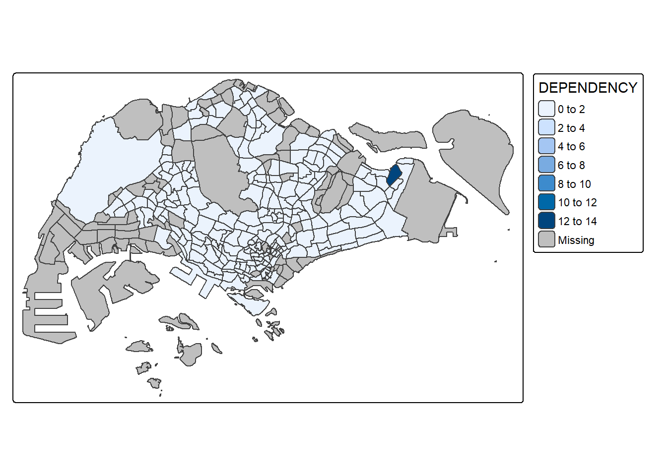
6.2. tmap Mapping
tm_shape(mpsz_pop2024) +
  tm_polygons(fill = "DEPENDENCY",
              fill.scale = tm_scale_intervals(
                style = "quantile",
                n = 5,
                values = "brewer.blues"),
              fill.legend = tm_legend(
                title = "Dependency ratio")) +
  tm_title("Distribution of Dependency Ratio by planning subzone") +
  tm_layout(frame = TRUE) +
  tm_borders(fill_alpha = 0.5) +
  tm_compass(type="8star", size = 2) +
  tm_scalebar() +
  tm_grid(alpha =0.2) +
  tm_credits("Source: Planning Sub-zone boundary from Urban Redevelopment Authorithy (URA)\n and Population data from Department of Statistics DOS",
             position = c("left", "bottom"))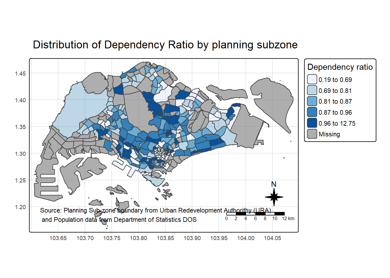
6.3. tmap with tm_shape() and tm_polygon()
tm_shape(mpsz_pop2024) +
  tm_polygons()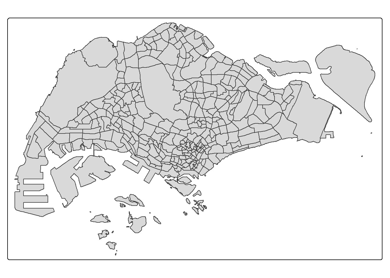
6.4. tmap with tm_polygon()
tm_shape(mpsz_pop2024)+ tm_polygons(fill = "DEPENDENCY")
6.5. Mapping with tm_fills and tm_borders()
Basic Choropleth with fill only
tm_shape(mpsz_pop2024) +
  tm_fill("DEPENDENCY")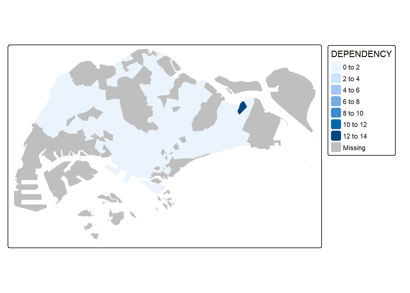
Adding Borders
tm_shape(mpsz_pop2024) +
  tm_fill("DEPENDENCY") +
  tm_borders()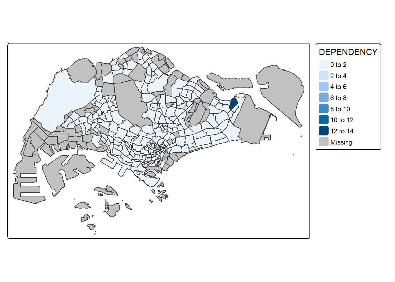
Customizing Borders
tm_shape(mpsz_pop2024) +
  tm_fill("DEPENDENCY") +
  tm_borders(col = "grey60", lwd = 0.1, lty = "dashed")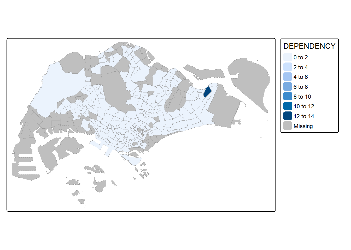
7. Data classification functions of tmap
7.1. Using inbuilt functions
tm_shape(mpsz_pop2024) +
  tm_polygons(fill = "DEPENDENCY",
              fill.scale = tm_scale_intervals(
                style = "quantile",
                n = 5)) +
  tm_borders(fill_alpha = 0.5)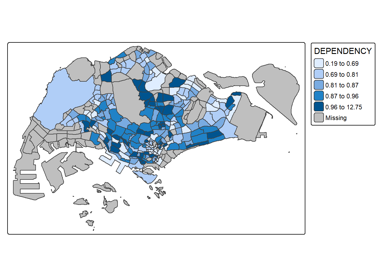
tm_shape(mpsz_pop2024) +
  tm_polygons(fill = "DEPENDENCY",
              fill.scale = tm_scale_intervals(
                style = "equal",
                n = 5)) +
  tm_borders(fill_alpha = 0.5)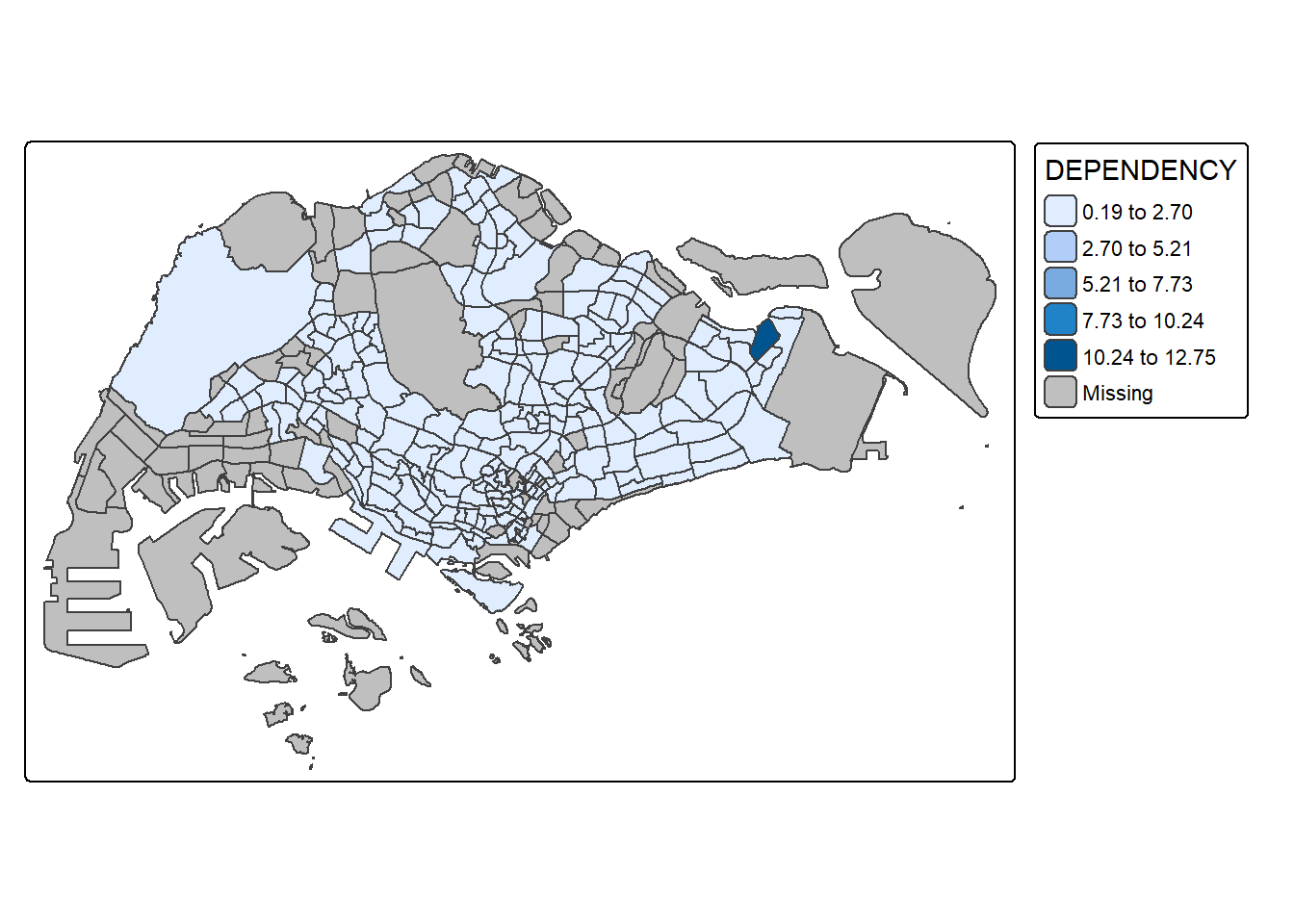
7.2. Plotting with custome break
Exploring the data
summary(mpsz_pop2024$DEPENDENCY) Min. 1st Qu. Median Mean 3rd Qu. Max. NA's
0.1905 0.7450 0.8377 0.8738 0.9366 12.7500 94 Plotting with custome breaks
tm_shape(mpsz_pop2024) +
  tm_polygons(fill = "DEPENDENCY",
              fill.scale = tm_scale_intervals(
                breaks = c(0, 0.60, 0.70, 0.80, 0.90, 1.00))) +
  tm_borders(fill_alpha = 0.5)
Warning: Values have found that are higher than the highest break. They are
assigned to the highest interval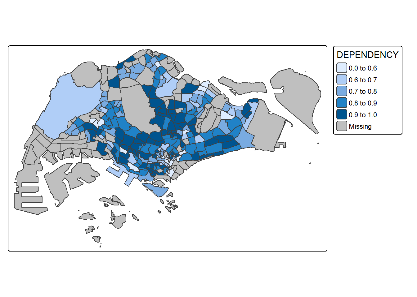
8. Colour Scheme
8.1. Using Colour Brewer Pallete
tm_shape(mpsz_pop2024) +
  tm_polygons(fill = "DEPENDENCY",
              fill.scale = tm_scale_intervals(
                style = "quantile",
                n = 5,
                values = "brewer.greens")) +
  tm_borders(fill_alpha = 0.5)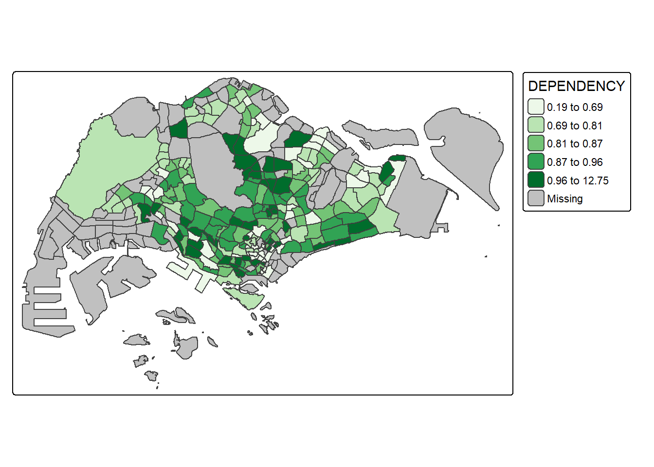
tm_shape(mpsz_pop2024) +
  tm_polygons(fill = "DEPENDENCY",
              fill.scale = tm_scale_intervals(
                style = "quantile",
                n = 5,
                values = "-brewer.greens")) +
  tm_borders(fill_alpha = 0.5)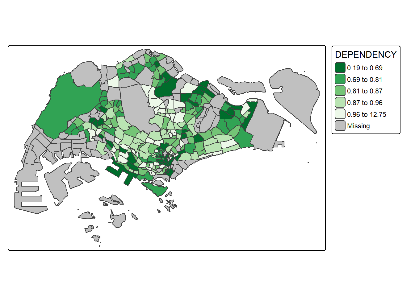
8.2. Cartographic Furniture
tm_shape(mpsz_pop2024) +
  tm_polygons(fill = "DEPENDENCY",
              fill.scale = tm_scale_intervals(
                style = "quantile",
                n = 5)) +
  tm_borders(fill_alpha = 0.5) +
  tm_compass(type="8star", size = 2) +
  tm_scalebar() +
  tm_grid(lwd = 0.1, alpha = 0.2) +
  tm_credits("Source: data.gov.sg & singstat",
             position = c("left", "bottom"))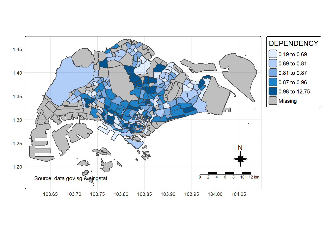
9. Map Layout
9.1. Map Legend
tm_shape(mpsz_pop2024) +
  tm_polygons(fill = "DEPENDENCY",
              fill.scale = tm_scale_intervals(
                style = "quantile",
                n = 5),
              fill.legend = tm_legend(
                title = "Dependency ratio")) +
  tm_pos_auto_in() +
  tm_borders(fill_alpha = 0.5) +
  tm_compass(type="8star", size = 2) +
  tm_scalebar() +
  tm_grid(lwd = 0.1, alpha = 0.2) +
  tm_credits("Source: data.gov.sg & singstat",
             position = c("left", "bottom"))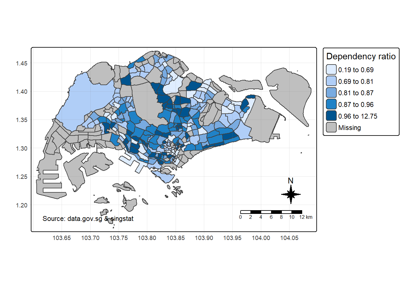
9.2. Map Style
tm_shape(mpsz_pop2024) +
  tm_polygons(fill = "DEPENDENCY",
              fill.scale = tm_scale_intervals(
                style = "quantile",
                n = 5,
                values = "-brewer.greens")) +
  tm_borders(fill_alpha = 0.5) +
  tmap_style("natural")
style set to "natural"other available styles are: "white" (tmap default), "gray", "cobalt", "albatross", "beaver", "bw", "classic", "watercolor"tmap v3 styles: "v3" (tmap v3 default), "gray_v3", "natural_v3", "cobalt_v3", "albatross_v3", "beaver_v3", "bw_v3", "classic_v3", "watercolor_v3"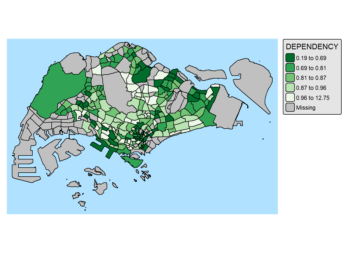
10. Drawing Small Choropleth maps
10.1. By assigning multiple values to at least one of the aesthetic arguments
tm_shape(mpsz_pop2024) +
  tm_polygons(
    fill = c("YOUNG", "AGED"),
    fill.legend =
      tm_legend(position = tm_pos_in(
        "right", "bottom")),
    fill.scale = tm_scale_intervals(
      style = "equal",
      n = 5,
      values = "brewer.blues")) +
  tm_borders(fill_alpha = 0.5) +
  tmap_style("natural")
style set to "natural"other available styles are: "white" (tmap default), "gray", "cobalt", "albatross", "beaver", "bw", "classic", "watercolor"tmap v3 styles: "v3" (tmap v3 default), "gray_v3", "natural_v3", "cobalt_v3", "albatross_v3", "beaver_v3", "bw_v3", "classic_v3", "watercolor_v3"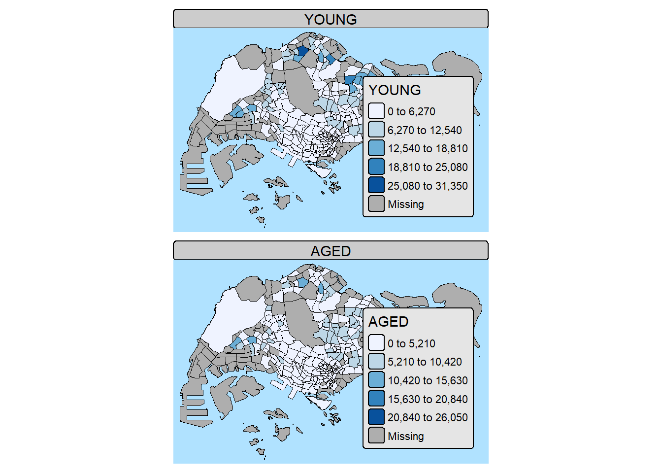
10.2. By arrange multiples choropleth maps in a grid layout
youngmap <- tm_shape(mpsz_pop2024)+
  tm_polygons(fill = "YOUNG",
              fill.legend = tm_legend(
                position = tm_pos_in(
                  "right", "bottom"),
                  item.height = 0.8),
              fill.scale = tm_scale_intervals(
                style = "quantile",
                values = "brewer.blues")) +
  tm_borders(fill_alpha = 0.5) +
  tm_title("Distribution of young population")

agedmap <- tm_shape(mpsz_pop2024)+
  tm_polygons(fill = "AGED",
              fill.legend = tm_legend(
                position = tm_pos_in(
                  "right", "bottom"),
                item.height = 0.8),
              fill.scale = tm_scale_intervals(
              style = "quantile",
              values = "brewer.blues")) +
  tm_borders(fill_alpha = 0.5) +
  tm_title("Distribution of aged population")

tmap_arrange(youngmap, agedmap, asp=1, ncol=2)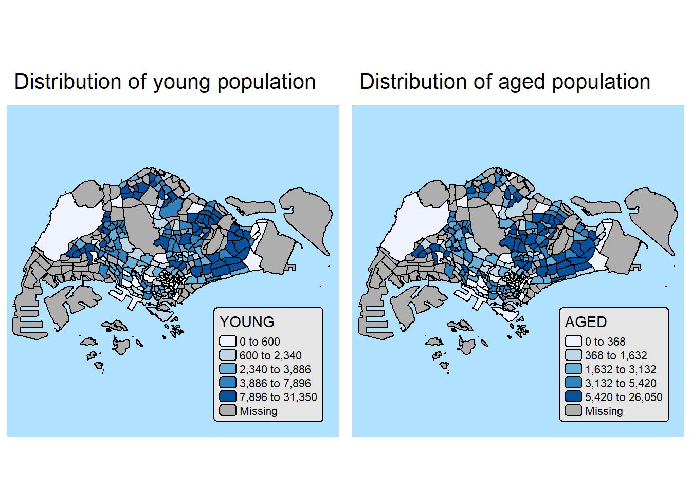
10.3. By defining group-by variable in tm_facets()
tm_shape(mpsz_pop2024) +
  tm_fill(fill = "DEPENDENCY",
          fill.scale = tm_scale_intervals(
            style = "quantile",
            values = "brewer.blues")) +
  tm_facets(by = "REGION_N",
            nrow = 2,
            ncols = 3,
            free.coords=TRUE,
            drop.units=TRUE) +
  tm_layout(legend.show = TRUE,
            title.position = c("center", "center"),
            title.size = 20) +
  tm_borders(fill_alpha = 0.5)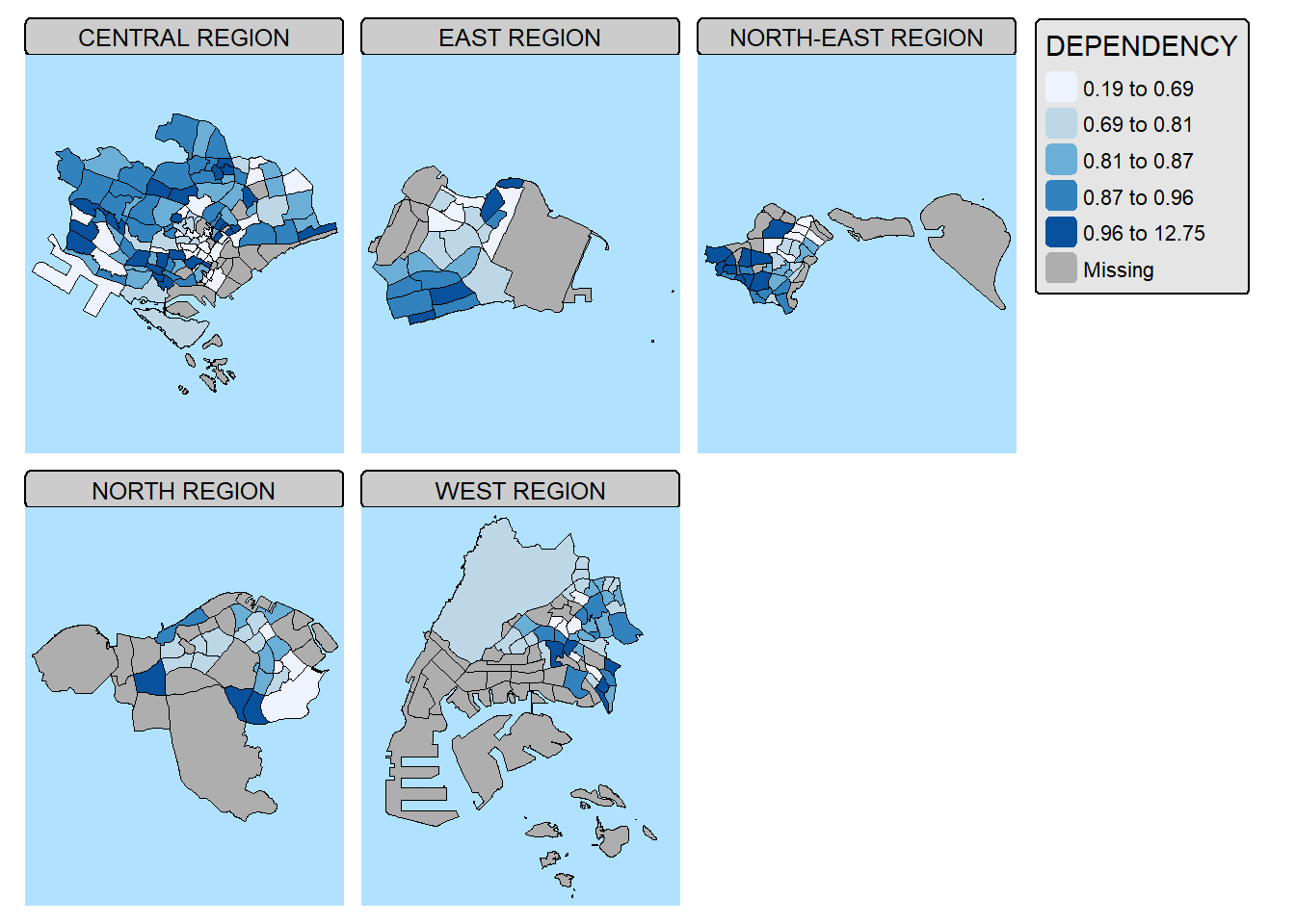
11. Mappping Spatial Object Meeting a Selection Criterion
Instead of creating small multiple choropleth map, you can also use filter() of dplyr package to select geographical area of interest and plot a choropleth map focus only on the selected region.
mpsz_pop2024 %>%
  filter(REGION_N == "CENTRAL REGION") %>%
  tm_shape() +
  tm_polygons(fill = "DEPENDENCY",
              fill.scale = tm_scale_intervals(
                style = "quantile",
                values = "brewer.greens"),
              fill.legend = tm_legend()) +
  tm_borders(fill_alpha = 0.5)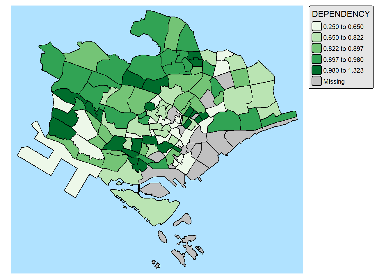
12. Complementing Thematic Map with Statistical Chart
Maps and statistical charts complement each other by visually representing different aspects of the same data, offering a more comprehensive understanding. Maps excel at showing spatial relationships and geographical patterns, while charts effectively display numerical data, trends, and comparisons. Combining both allows for a more insightful and engaging data narrative, especially when dealing with spatial data that also has quantifiable characteristics.
With tmap, statistical chart and be incorporate into the map visualisation by using fill.chat argument of map layers and legend chart feature as shown in the code chunk below.
mpsz_pop2024 %>%
  filter(REGION_N == "CENTRAL REGION") %>%
  tm_shape() +
  tm_polygons(fill = "DEPENDENCY",
              fill.scale = tm_scale_intervals(
                style = "quantile",
                values = "brewer.greens"),
              fill.legend = tm_legend(),
              fill.chart = tm_chart_box()) +
  tm_borders() +
  tm_layout(asp = 0.8)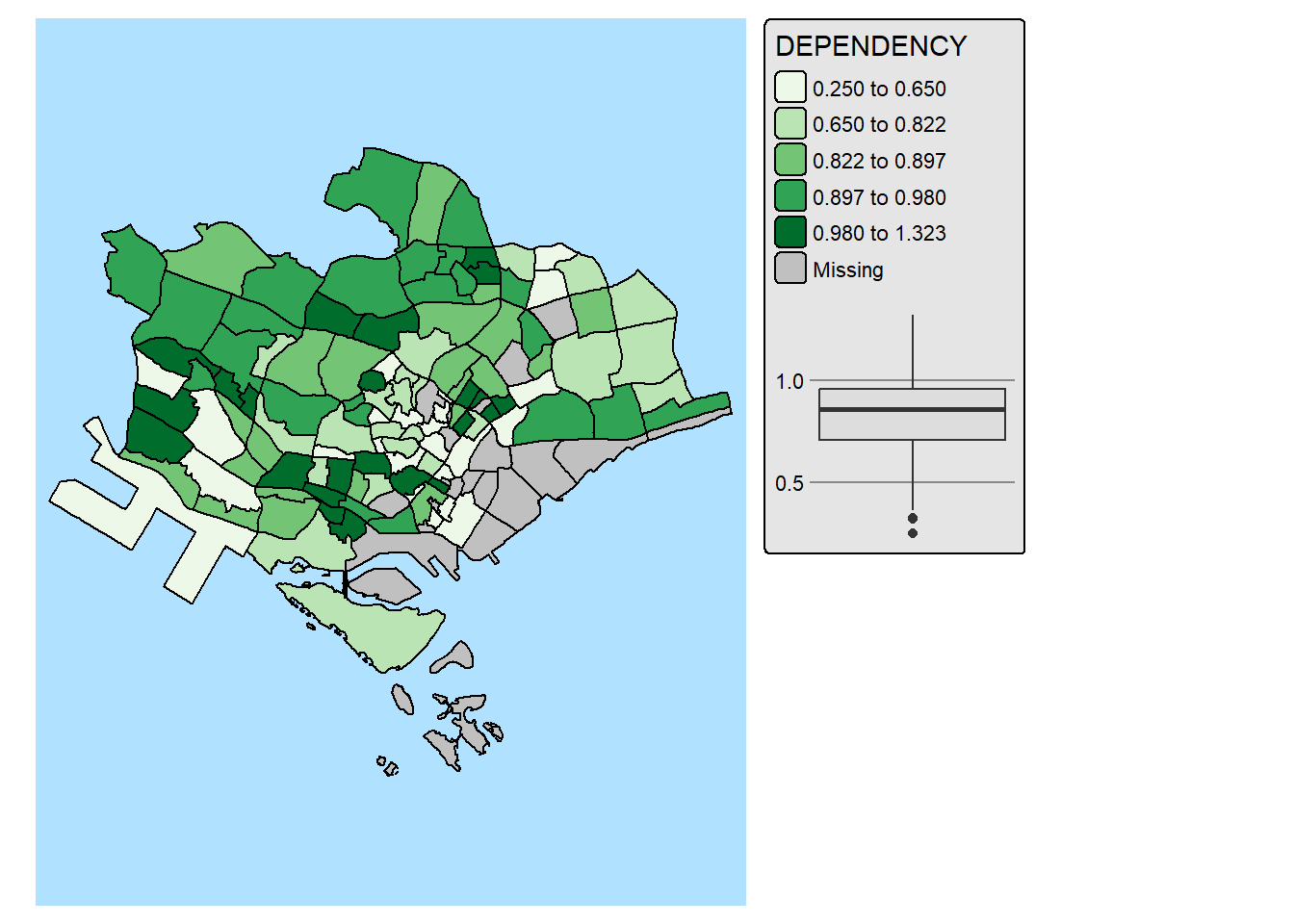
In the code chunk below, We improve the visual representation further by highlighting and lebaling the outliers on the choropleth map.
mpsz_selected <- mpsz_pop2024 %>%
  filter(REGION_N == "CENTRAL REGION")

stats <- boxplot.stats(mpsz_selected$DEPENDENCY)

outlier_vals <- stats$out

outlier_sf <- mpsz_selected[mpsz_selected$DEPENDENCY %in% outlier_vals, ]

tm_shape(mpsz_selected) +
  tm_polygons(fill = "DEPENDENCY",
          fill.scale = tm_scale_intervals(
            style = "quantile",
            values = "brewer.blues"),
          fill.legend = tm_legend(),
          fill.chart = tm_chart_box()) +
  tm_borders(fill_alpha = 0.5) +
tm_shape(outlier_sf) +
  tm_borders(col = "red", lwd = 2) +
  tm_text("SUBZONE_N", col = "red", size = 0.7) +
  tm_layout(asp = 0.8)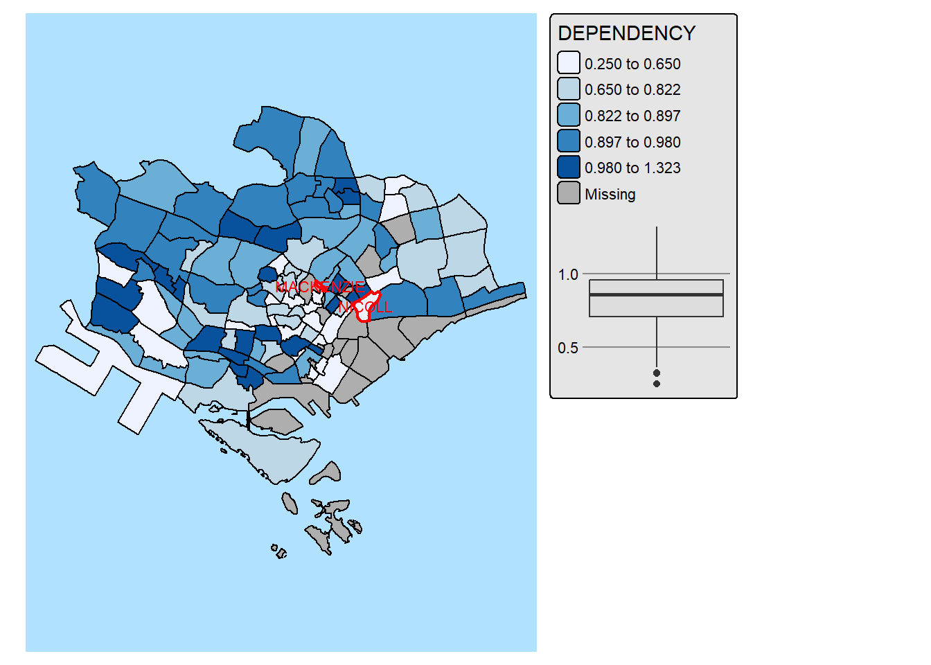
13. Create Interactive Mapping
region_selected <- mpsz_pop2024 %>%
  filter(REGION_N == "CENTRAL REGION")
region_bbox <- st_bbox(region_selected)

stats <- boxplot.stats(region_selected$DEPENDENCY)
outlier_vals <- stats$out
outlier_sf <- region_selected[region_selected$DEPENDENCY %in% outlier_vals, ]

tmap_mode("view")
ℹ tmap mode set to "view".tm_shape(region_selected,
bbox = region_bbox) +
tm_fill("DEPENDENCY",
id = "SUBZONE_N",
popup.vars = c(
"Name" = "SUBZONE_N",
"Dependency" = "DEPENDENCY")) +
tm_borders() +
tm_shape(outlier_sf) +
tm_borders(col = "red", lwd = 2)tmap_mode("plot")ℹ tmap mode set to "plot".The interactive map above is far from satisfactory. While we want to encourage users to engage and explore the interactive by zooming in and out of the study area freely. But, users might lost in the cyberspace with too much freedom to zoom-in and zoom-out.
To address this issue, set_zoom_limits argument can be used to limit the map extend users can zooming in and out of the map areas as shown below.
region_selected <- mpsz_pop2024 %>%
  filter(REGION_N == "CENTRAL REGION")
region_bbox <- st_bbox(region_selected)

stats <- boxplot.stats(region_selected$DEPENDENCY)
outlier_vals <- stats$out
outlier_sf <- region_selected[region_selected$DEPENDENCY %in% outlier_vals, ]

tmap_mode("view")
ℹ tmap mode set to "view".tm_shape(region_selected,
bbox = region_bbox) +
tm_fill("DEPENDENCY",
id = "SUBZONE_N",
popup.vars = c(
"Name" = "SUBZONE_N",
"Dependency" = "DEPENDENCY")) +
tm_borders() +
tm_shape(outlier_sf) +
tm_borders(col = "red", lwd = 2) +
tm_view(set_zoom_limits = c(12,14))