pacman::p_load(sf, terra, spatstat,
tmap, rvest, tidyverse)Hands-on Exercise 2A - First-order Spatial Point Patterns Analysis Methods
1.Overview
First-order Spatial Point Pattern Analysis (1st-SPPA) is a method used to study the spatial distribution and density of point-based phenomena—such as crime events, business locations, or public facilities—across a geographic area. Unlike higher-order analyses, 1st-SPPA focuses solely on individual point locations and their spread, without considering interactions between them. It helps identify where points are most concentrated, whether their distribution is uniform, and how widely they are dispersed. In this context, the chapter introduces hands-on techniques using the spatstat package to explore whether childcare centres in Singapore are randomly distributed, and if not, to pinpoint areas with higher concentrations.
2. Data
Child Care Services data from data.gov.sg, a point feature data providing both location and attribute information of childcare centres.
Master Plan 2019 Subzone Boundary (No Sea), a polygon feature data providing information of URA 2019 Master Plan Planning Subzone boundary data.
3. Installing and Loading R Packages
4. Importing and Wrangling Geospatial Datasets
Import the master plan subzone boundary
mpsz_sf <- st_read("data/MasterPlan2019SubzoneBoundaryNoSeaKML (1).kml") %>%
  st_zm(drop = TRUE, what = "ZM") %>% st_transform(crs = 3414)
Reading layer `URA_MP19_SUBZONE_NO_SEA_PL' from data source
`D:\ssinha8752\ISSS608-VAA\Hands-on_Ex\Hands-on_Ex02\data\MasterPlan2019SubzoneBoundaryNoSeaKML (1).kml'
using driver `KML'
Simple feature collection with 332 features and 2 fields
Geometry type: MULTIPOLYGON
Dimension: XY
Bounding box: xmin: 103.6057 ymin: 1.158699 xmax: 104.0885 ymax: 1.470775
Geodetic CRS: WGS 84Extract the Key attributes and KML descriptions
extract_kml_field <- function(html_text, field_name) {
  if (is.na(html_text) || html_text == "") return(NA_character_)
  page <- read_html(html_text)
  rows <- page %>% html_elements("tr")
  value <- rows %>%
    keep(~ html_text2(html_element(.x, "th")) == field_name) %>%
    html_element("td") %>%
    html_text2()
  if (length(value) == 0) NA_character_ else value
}
Clean the structure and subzone data
mpsz_sf <- mpsz_sf %>%
  mutate(
    REGION_N = map_chr(Description, extract_kml_field, "REGION_N"),
    PLN_AREA_N = map_chr(Description, extract_kml_field, "PLN_AREA_N"),
    SUBZONE_N = map_chr(Description, extract_kml_field, "SUBZONE_N"),
    SUBZONE_C = map_chr(Description, extract_kml_field, "SUBZONE_C")
  ) %>%
  select(-Name, -Description) %>%
  relocate(geometry, .after = last_col())
Filter out Non-Mainland subzones
mpsz_cl <- mpsz_sf %>%
  filter(SUBZONE_N != "SOUTHERN GROUP",
         PLN_AREA_N != "WESTERN ISLANDS",
         PLN_AREA_N != "NORTH-EASTERN ISLANDS")
Save the cleaned subzone
write_rds(mpsz_cl, "data/mpsz_cl.rds")Import the childcare services data
childcare_sf <- st_read("data/ChildCareServices.kml") %>%
  st_zm(drop = TRUE, what = "ZM") %>%
  st_transform(crs = 3414)
Reading layer `CHILDCARE' from data source
`D:\ssinha8752\ISSS608-VAA\Hands-on_Ex\Hands-on_Ex02\data\ChildCareServices.kml'
using driver `KML'
Simple feature collection with 1925 features and 2 fields
Geometry type: POINT
Dimension: XYZ
Bounding box: xmin: 103.6878 ymin: 1.247759 xmax: 103.9897 ymax: 1.462134
z_range: zmin: 0 zmax: 0
Geodetic CRS: WGS 84Validate the CRS Match
st_crs(mpsz_cl) == st_crs(childcare_sf)[1] TRUE4.1 Mapping Geospatial Datasets
DIY
library(sf)
library(ggplot2)
library(readr)

# Load cleaned subzone and childcare datasets
mpsz_cl <- read_rds("data/mpsz_cl.rds")
childcare_sf <- st_read("data/ChildCareServices.kml") %>%
  st_zm(drop = TRUE, what = "ZM") %>%
  st_transform(crs = st_crs(mpsz_cl))  # Ensure same CRS
Reading layer `CHILDCARE' from data source
`D:\ssinha8752\ISSS608-VAA\Hands-on_Ex\Hands-on_Ex02\data\ChildCareServices.kml'
using driver `KML'
Simple feature collection with 1925 features and 2 fields
Geometry type: POINT
Dimension: XYZ
Bounding box: xmin: 103.6878 ymin: 1.247759 xmax: 103.9897 ymax: 1.462134
z_range: zmin: 0 zmax: 0
Geodetic CRS: WGS 84# Create the map
ggplot() +
geom_sf(data = mpsz_cl, fill = "gray", color = "black", size = 0.2) +
geom_sf(data = childcare_sf, color = "black", size = 1.2, alpha = 0.7) +
labs(title = "Childcare Services Across Singapore Subzones",
subtitle = "All layers aligned to EPSG:3414 (SVY21)",
caption = "Source: URA Master Plan & Data.gov.sg") +
theme_minimal()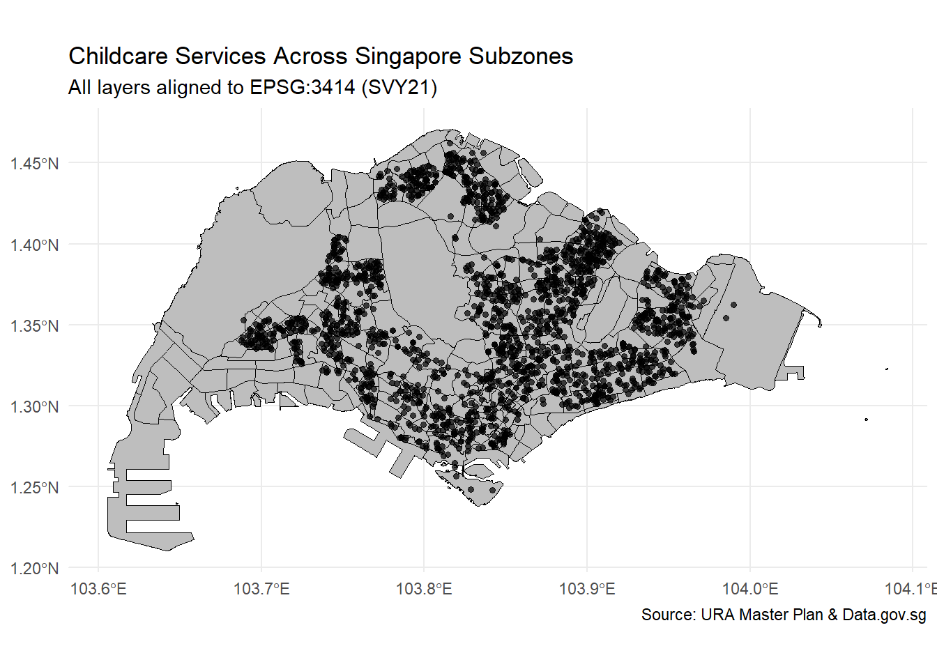
Interactive mapping with tmap()
tmap_mode("view")ℹ tmap mode set to "view".tm_shape(childcare_sf) +
tm_dots()Registered S3 method overwritten by 'jsonify':
method from
print.json jsonliteSwitching back to plot
tmap_mode("plot")ℹ tmap mode set to "plot".5. Geospatial Data Wrangling
5.1 Converting sf data frames to ppp class
spatstat requires the point event data in ppp object form. The code chunk below uses [as.ppp()] of spatstat package to convert childcare_sf to ppp format.
childcare_ppp <- as.ppp(childcare_sf)class(childcare_ppp)[1] "ppp"summary(childcare_ppp)Marked planar point pattern: 1925 points
Average intensity 2.417323e-06 points per square unit
Coordinates are given to 11 decimal places
Mark variables: Name, Description
Summary:
Name Description
Length:1925 Length:1925
Class :character Class :character
Mode :character Mode :character
Window: rectangle = [11810.03, 45404.24] x [25596.33, 49300.88] units
(33590 x 23700 units)
Window area = 796335000 square units5.2 Creating owin object
it is a good practice to confine the analysis with a geographical area like Singapore boundary. In spatstat, an object called owin is specially designed to represent this polygonal region.
The code chunk below, as.owin() of spatstat is used to covert mpsz_sf into owin object of spatstat.
sg_owin <- as.owin(mpsz_cl)class(sg_owin)[1] "owin"plot(sg_owin)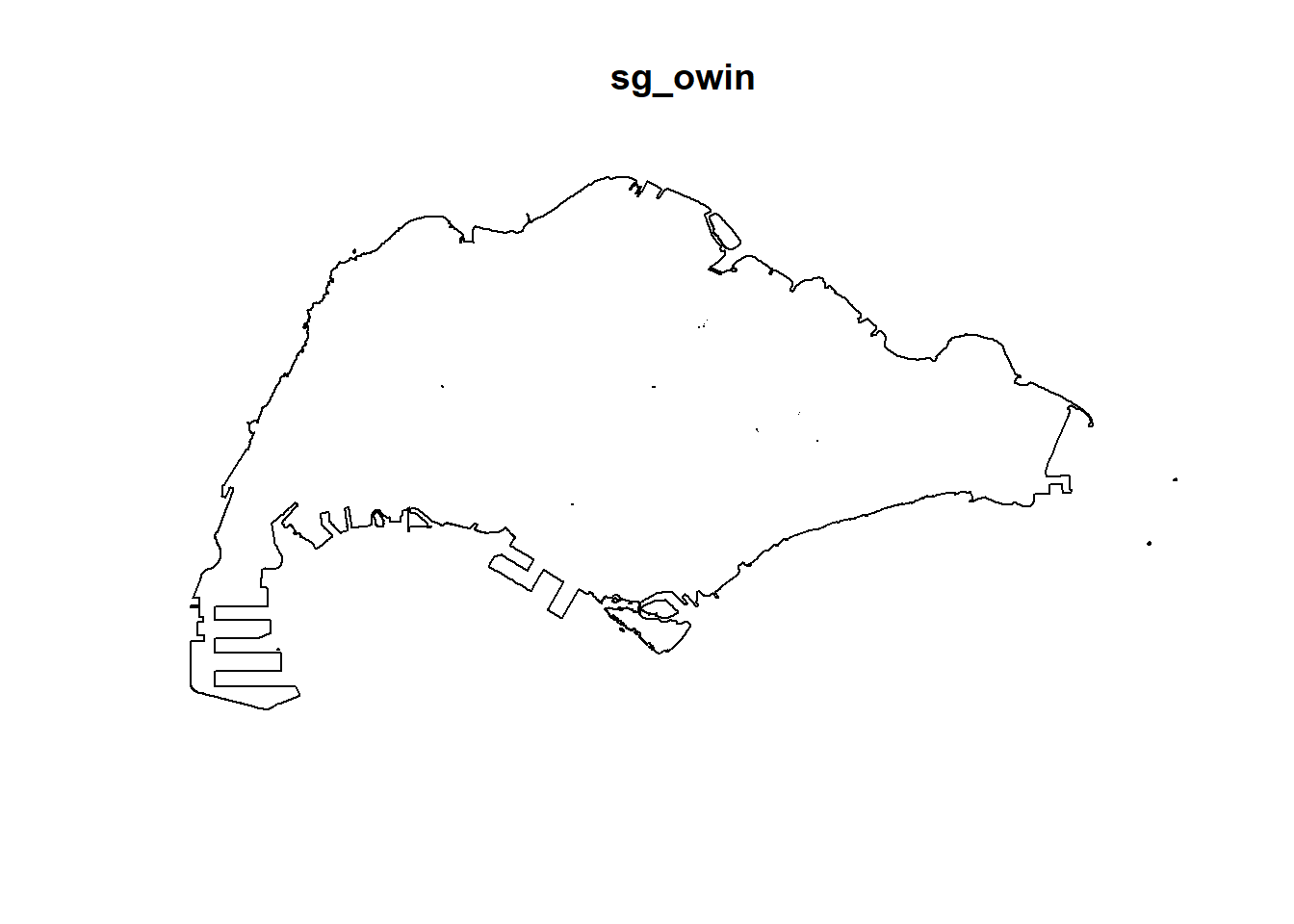
5.3 Combining point events object and owin object
Extraction the childcare events that are located within Singapore by using the code chunk below.
childcareSG_ppp = childcare_ppp[sg_owin]The output object combined both the point and polygon feature in one ppp object class as shown below.
childcareSG_pppMarked planar point pattern: 1925 points
Mark variables: Name, Description
window: polygonal boundary
enclosing rectangle: [2667.54, 55941.94] x [21448.47, 50256.33] units6. Clark-Evan Test for Nearest Neighbour Analysis
Nearest Neighbor Analysis (NNA) is a spatial statistics method that calculates the average distance between each point and its closest neighbor to determine if a pattern of points is clustered, dispersed, or randomly distributed.
Clark-Evans test is a specific statistical method used within NNA to quantify whether a point pattern is clustered, random, or uniformly spaced, using the Clark-Evans aggregation index (R) to describe this pattern. NNA provides a numerical value that describes the degree of clustering or regularity, and the Clark-Evans test calculates a specific index (R) for this purpose
6.1 Perform Clark Evans Test without CSR
library(spatstat.explore)clarkevans.test(childcareSG_ppp,
correction="none",
clipregion="sg_owin",
alternative=c("clustered"))
    Clark-Evans test
    No edge correction
    Z-test

data:  childcareSG_ppp
R = 0.53532, p-value < 2.2e-16
alternative hypothesis: clustered (R < 1)
Statistical Conclusion - Based on the Clark-Evans test, the observed R value of 0.53532 and a p-value less than 2.2e-16 provide strong statistical evidence that the distribution of childcare services is significantly clustered rather than randomly distributed.
Business Communication - The spatial analysis reveals that childcare services in Singapore are concentrated in specific areas, rather than evenly or randomly distributed across the region. This clustering may indicate oversupply in certain neighborhoods and underserved regions elsewhere. For urban planners, policymakers, or service providers, this insight highlights the need to reassess location strategies to ensure equitable access to childcare services citywide.
###6.2 Clark Exans Test with CSR
clarkevans.test(childcareSG_ppp,
                correction="none",
                clipregion="sg_owin",
                alternative=c("clustered"),
                method="MonteCarlo",
                nsim=99)
    Clark-Evans test
    No edge correction
    Monte Carlo test based on 99 simulations of CSR with fixed n

data:  childcareSG_ppp
R = 0.53532, p-value = 0.01
alternative hypothesis: clustered (R < 1)[Statistical Conclusion -] - The Clark-Evans test with Monte Carlo simulation yields an R value of 0.53532 and a p-value of 0.01. This provides strong evidence against the null hypothesis of random distribution. We conclude that the spatial distribution of childcare services is significantly clustered.
[Business Conclusion -] The spatial analysis reveals that childcare services in Singapore are not randomly distributed, but rather clustered in specific areas. This clustering may indicate oversupply in certain neighborhoods, while other regions may be underserved. For urban planners, service providers, and policymakers, this insight highlights the need to reassess location strategies to ensure equitable access to childcare services across the city. Strategic redistribution or expansion into underserved zones could improve service coverage and community satisfaction.
7. Kernel Density Estimation Method
Kernel Density Estimation (KDE) is a valuable tool for visualising and analyzing first-order spatial point patterns. It is widely considered a method within Exploratory Spatial Data Analysis (ESDA) because it’s used to visualize and understand spatial data patterns by transforms discrete point data (like locations of childcare service, crime incidents or disease cases) into continuous density surfaces that reveal clusters and variations in event occurrences, without making prior assumptions about data distribution. It helps to begin understanding data distribution, identify hotspots, and explore relationships between spatial variables before performing more rigorous analysis.
7.1 Automatic Bandwidth Selection
kde_SG_diggle <- density(
  childcareSG_ppp,
  sigma = bw.diggle,
  edge = TRUE,
  kernel = "gaussian"
)plot(kde_SG_diggle)
summary(kde_SG_diggle)real-valued pixel image
128 x 128 pixel array (ny, nx)
enclosing rectangle: [2667.538, 55941.94] x [21448.47, 50256.33] units
dimensions of each pixel: 416 x 225.0614 units
Image is defined on a subset of the rectangular grid
Subset area = 669941961.12249 square units
Subset area fraction = 0.437
Pixel values (inside window):
range = [-6.584123e-21, 3.063698e-05]
integral = 1927.788
mean = 2.877545e-06Retrieving the bandwidth value
bw <- bw.diggle(childcareSG_ppp)
bw
sigma
295.9712 7.2 Rescalling the KDE Values
childcareSG_ppp_km <- rescale.ppp(
  childcareSG_ppp, 1000, "km")
With density() -
kde_childcareSG_km <- density(childcareSG_ppp_km,
                              sigma=bw.diggle,
                              edge=TRUE,
kernel="gaussian")plot(kde_childcareSG_km)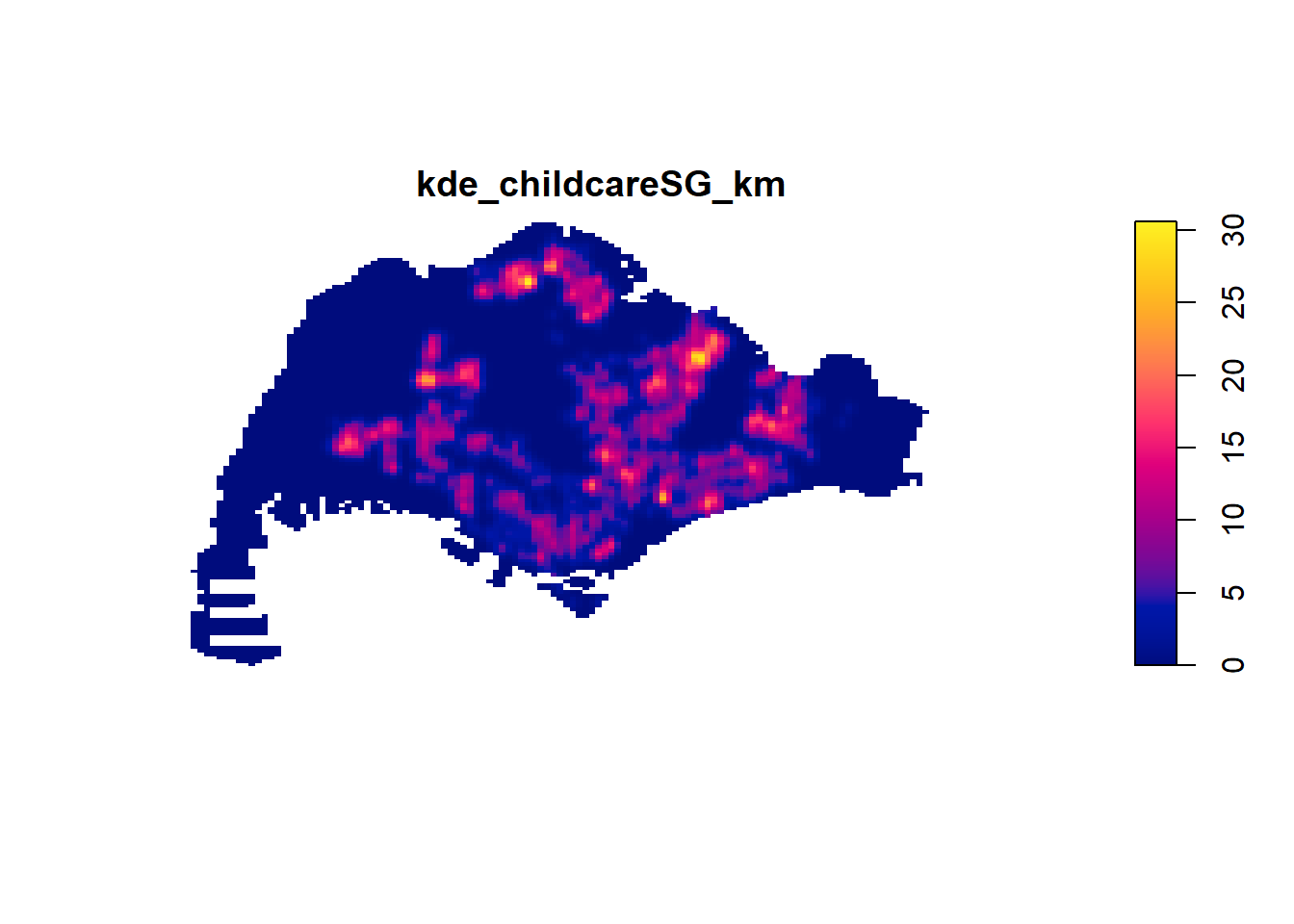
7.3 Working with different automatic badwidth methods
Cross-validation based; tends to be broader
bw.CvL(childcareSG_ppp_km) sigma
4.357209 Based on Scott’s rule; anisotropic
bw.scott(childcareSG_ppp_km) sigma.x sigma.y
2.159749 1.396455 Preferred for tight clusters
bw.ppl(childcareSG_ppp_km) sigma
0.378997 Best for detecting single tight clusters
bw.diggle(childcareSG_ppp_km) sigma
0.2959712 Computing KDE with bw.ppl() and comparing -
kde_childcareSG.ppl <- density(childcareSG_ppp_km,
                               sigma=bw.ppl,
                               edge=TRUE,
                               kernel="gaussian")
par(mfrow=c(1,2))
plot(kde_childcareSG_km, main = "bw.diggle")
plot(kde_childcareSG.ppl, main = "bw.ppl")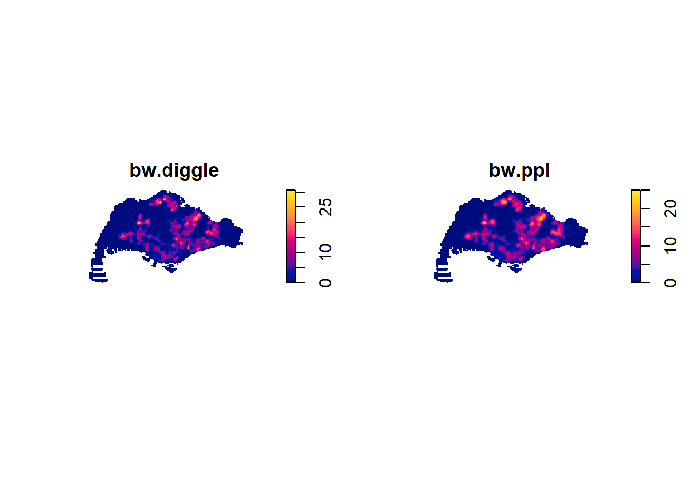
7.4 Working with different kernel methods
par(mfrow=c(2,2))
plot(density(childcareSG_ppp_km,
             sigma=0.2959712,
             edge=TRUE,
             kernel="gaussian"),
     main="Gaussian")
plot(density(childcareSG_ppp_km,
             sigma=0.2959712,
             edge=TRUE,
             kernel="epanechnikov"),
     main="Epanechnikov")
plot(density(childcareSG_ppp_km,
             sigma=0.2959712,
             edge=TRUE,
             kernel="quartic"),
     main="Quartic")
plot(density(childcareSG_ppp_km,
             sigma=0.2959712,
             edge=TRUE,
             kernel="disc"),
     main="Disc")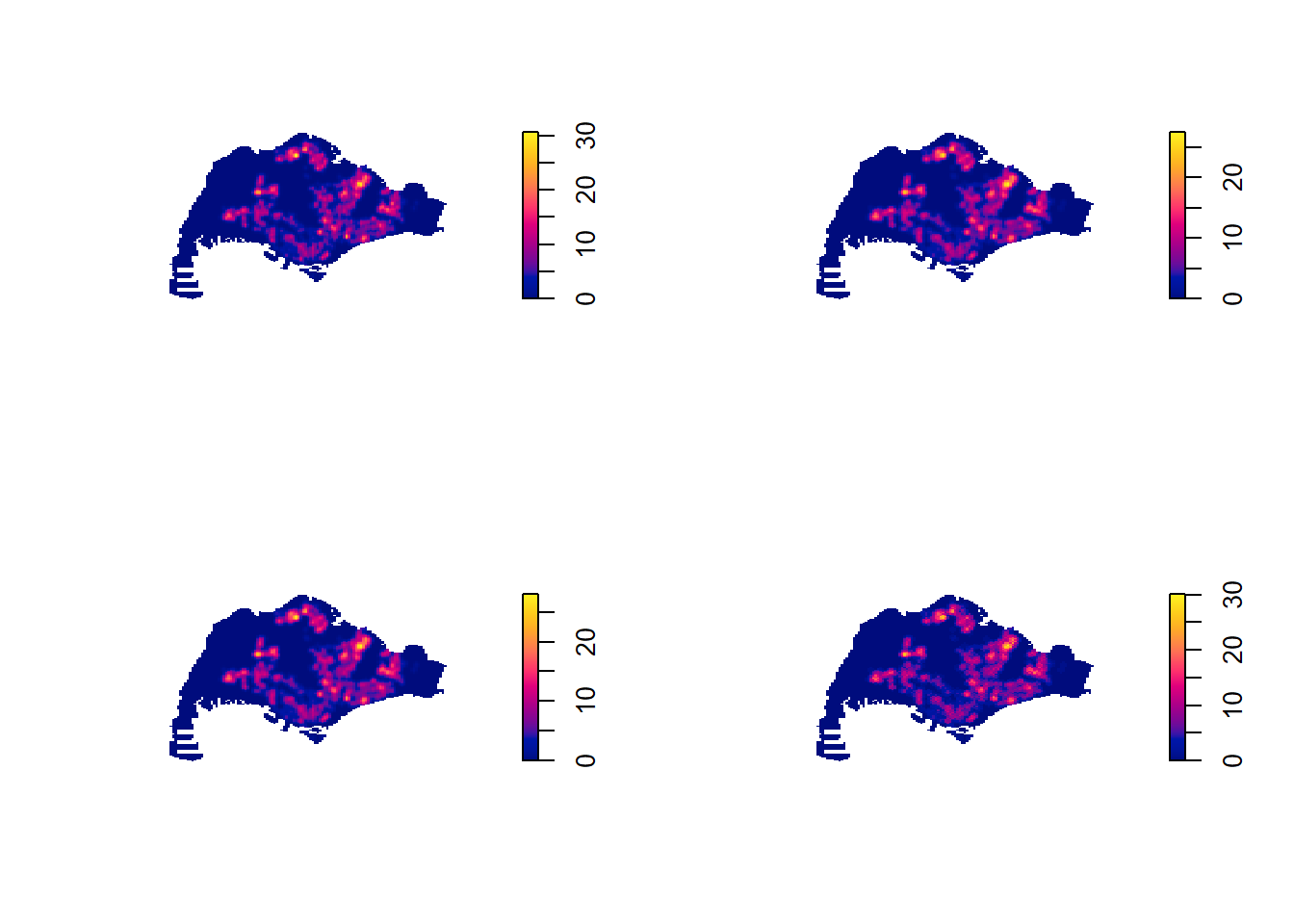
8.Fixed and Adaptive KDE
8.1 Computing KDE by using fixed bandwidth
kde_childcareSG_fb <- density(childcareSG_ppp_km,
                              sigma=0.6,
                              edge=TRUE,
                              kernel="gaussian")
plot(kde_childcareSG_fb)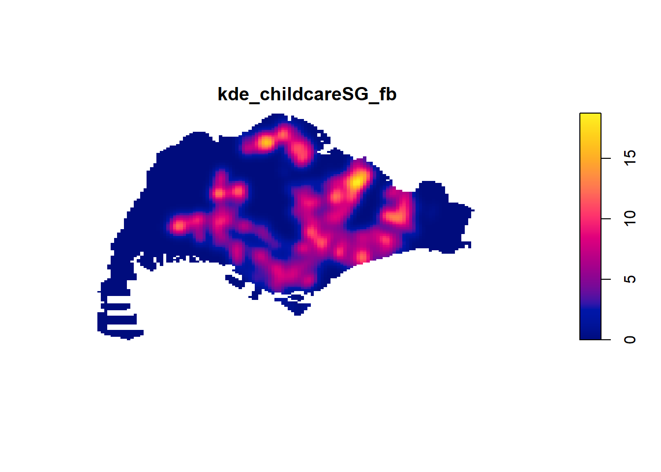
8.2 Computing KDE by using adaptive bandwidth
kde_childcareSG_ab <- adaptive.density(
  childcareSG_ppp_km,
  method="kernel")
plot(kde_childcareSG_ab)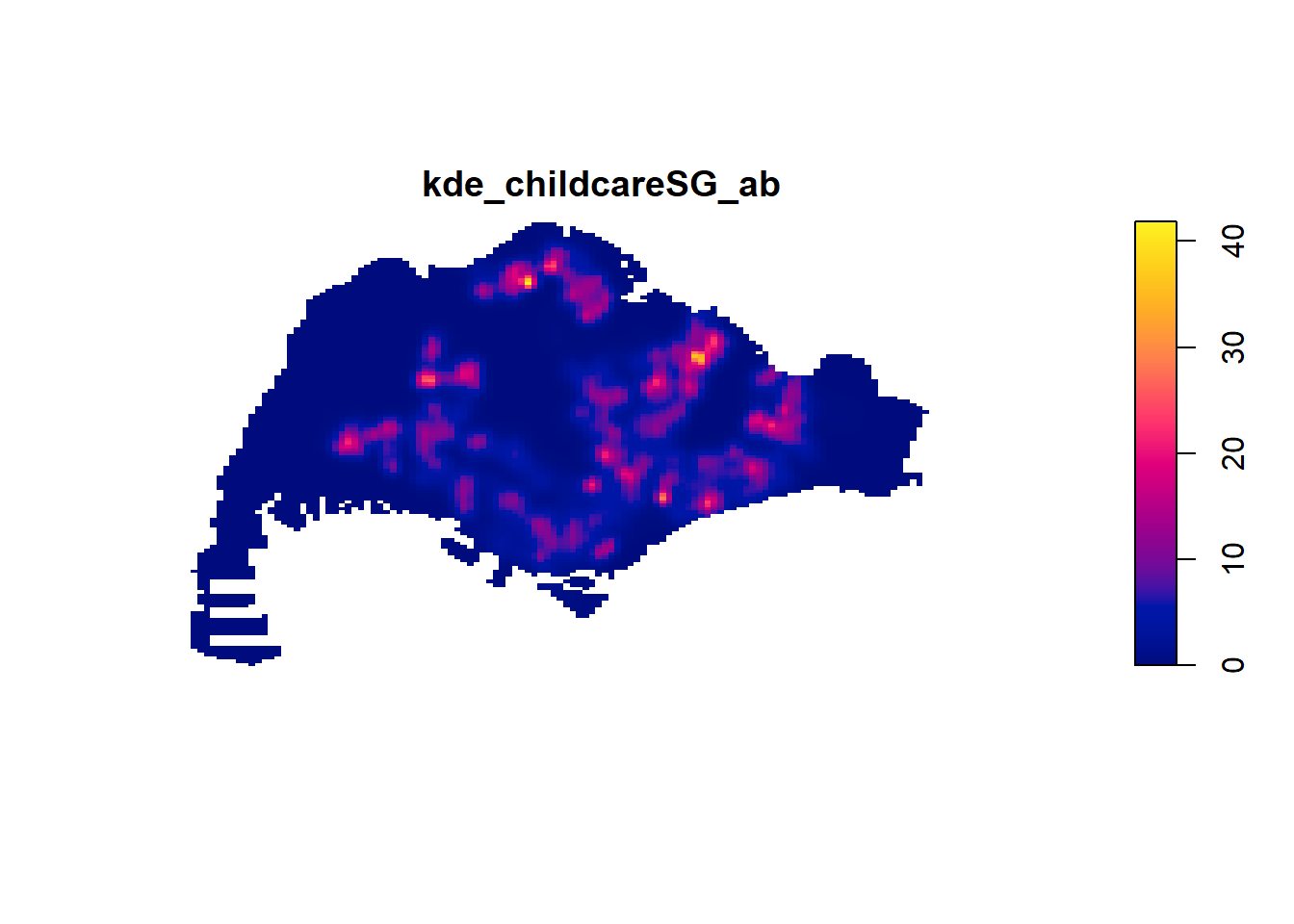
9. Plotting cartographic quality KDE map
9.1 Converting gridded output into raster
kde_childcareSG_bw_terra <- rast(kde_childcareSG_km)class(kde_childcareSG_bw_terra)[1] "SpatRaster"
attr(,"package")
[1] "terra"kde_childcareSG_bw_terraclass : SpatRaster
size : 128, 128, 1 (nrow, ncol, nlyr)
resolution : 0.4162063, 0.2250614 (x, y)
extent : 2.667538, 55.94194, 21.44847, 50.25633 (xmin, xmax, ymin, ymax)
coord. ref. :
source(s) : memory
name : lyr.1
min value : -5.824417e-15
max value : 3.063698e+01
unit : km 9.2 Assigning projection systems
crs(kde_childcareSG_bw_terra) <- "EPSG:3414"look at the properties of kde_childcareSG_bw_raster RasterLayer.
kde_childcareSG_bw_terraclass : SpatRaster
size : 128, 128, 1 (nrow, ncol, nlyr)
resolution : 0.4162063, 0.2250614 (x, y)
extent : 2.667538, 55.94194, 21.44847, 50.25633 (xmin, xmax, ymin, ymax)
coord. ref. : SVY21 / Singapore TM (EPSG:3414)
source(s) : memory
name : lyr.1
min value : -5.824417e-15
max value : 3.063698e+01
unit : km 9.3 Plotting KDE map with tmap
We will display the raster in cartographic quality map using tmap package.
tm_shape(kde_childcareSG_bw_terra) +
  tm_raster(col.scale =
              tm_scale_continuous(
                values = "viridis"),
            col.legend = tm_legend(
            title = "Density values",
            title.size = 0.7,
            text.size = 0.7,
            bg.color = "white",
            bg.alpha = 0.7,
            position = tm_pos_in(
              "right", "bottom"),
            frame = TRUE)) +
  tm_graticules(labels.size = 0.7) +
  tm_compass() +
  tm_layout(scale = 1.0)
[plot mode] legend/component: Some components or legends are too "high" and are
therefore rescaled.
ℹ Set the tmap option `component.autoscale = FALSE` to disable rescaling.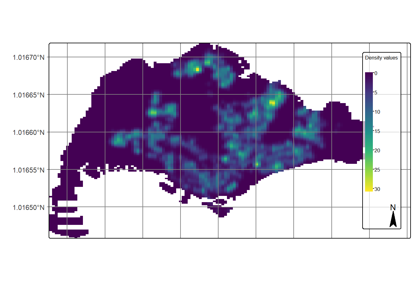
10. First Order SPPA at the Planning Subzone Level
10.1 Geospatial data wrangling
10.1.1 Extracting study area The code chunk below will be used to extract the target planning areas.
pg <- mpsz_cl %>%
  filter(PLN_AREA_N == "PUNGGOL")
tm <- mpsz_cl %>%
  filter(PLN_AREA_N == "TAMPINES")
ck <- mpsz_cl %>%
  filter(PLN_AREA_N == "CHOA CHU KANG")
jw <- mpsz_cl %>%
  filter(PLN_AREA_N == "JURONG WEST")
It is always a good practice to review the extracted areas. The code chunk below will be used to plot the extracted planning areas.
par(mfrow=c(2,2))
plot(st_geometry(pg), main = "Ponggol")
plot(st_geometry(tm), main = "Tampines")
plot(st_geometry(ck), main = "Choa Chu Kang")
plot(st_geometry(jw), main = "Jurong West")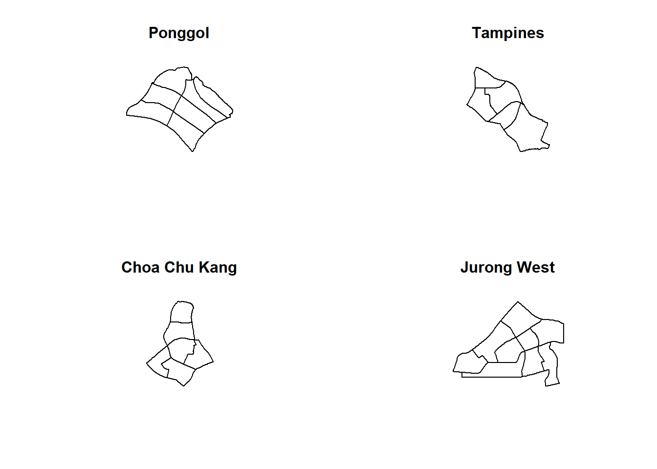
10.1.2 Creating owin object Now, we will convert these sf objects into owin objects that is required by spatstat.
pg_owin = as.owin(pg)
tm_owin = as.owin(tm)
ck_owin = as.owin(ck)
jw_owin = as.owin(jw)
10.1.3 Combining point events object and owin object
childcare_pg_ppp = childcare_ppp[pg_owin]
childcare_tm_ppp = childcare_ppp[tm_owin]
childcare_ck_ppp = childcare_ppp[ck_owin]
childcare_jw_ppp = childcare_ppp[jw_owin]
Next, rescale.ppp() function is used to trasnform the unit of measurement from metre to kilometre.
childcare_pg_ppp.km = rescale.ppp(childcare_pg_ppp, 1000, "km")
childcare_tm_ppp.km = rescale.ppp(childcare_tm_ppp, 1000, "km")
childcare_ck_ppp.km = rescale.ppp(childcare_ck_ppp, 1000, "km")
childcare_jw_ppp.km = rescale.ppp(childcare_jw_ppp, 1000, "km")
The code chunk below is used to plot these four study areas and the locations of the childcare centres.
par(mfrow=c(2,2))
plot(unmark(childcare_pg_ppp.km),
  main="Punggol")
plot(unmark(childcare_tm_ppp.km),
  main="Tampines")
plot(unmark(childcare_ck_ppp.km),
  main="Choa Chu Kang")
plot(unmark(childcare_jw_ppp.km),
  main="Jurong West")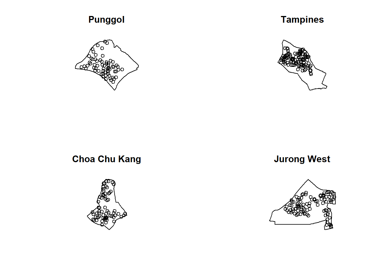
10.2 Clark and Evans Test
10.2.1 Choa Chu Kang planning area In the code chunk below, clarkevans.test() of spatstat is used to performs Clark-Evans test of aggregation for childcare centre in Choa Chu Kang planning area.
clarkevans.test(childcare_ck_ppp,
                correction="none",
                clipregion=NULL,
                alternative=c("two.sided"),
                nsim=999)
    Clark-Evans test
    No edge correction
    Z-test

data:  childcare_ck_ppp
R = 0.84097, p-value = 0.008866
alternative hypothesis: two-sidedclarkevans.test(childcare_tm_ppp,
correction="none",
clipregion=NULL,
alternative=c("two.sided"),
nsim=999)
Clark-Evans test
No edge correction
Z-test
data: childcare_tm_ppp
R = 0.66817, p-value = 6.58e-12
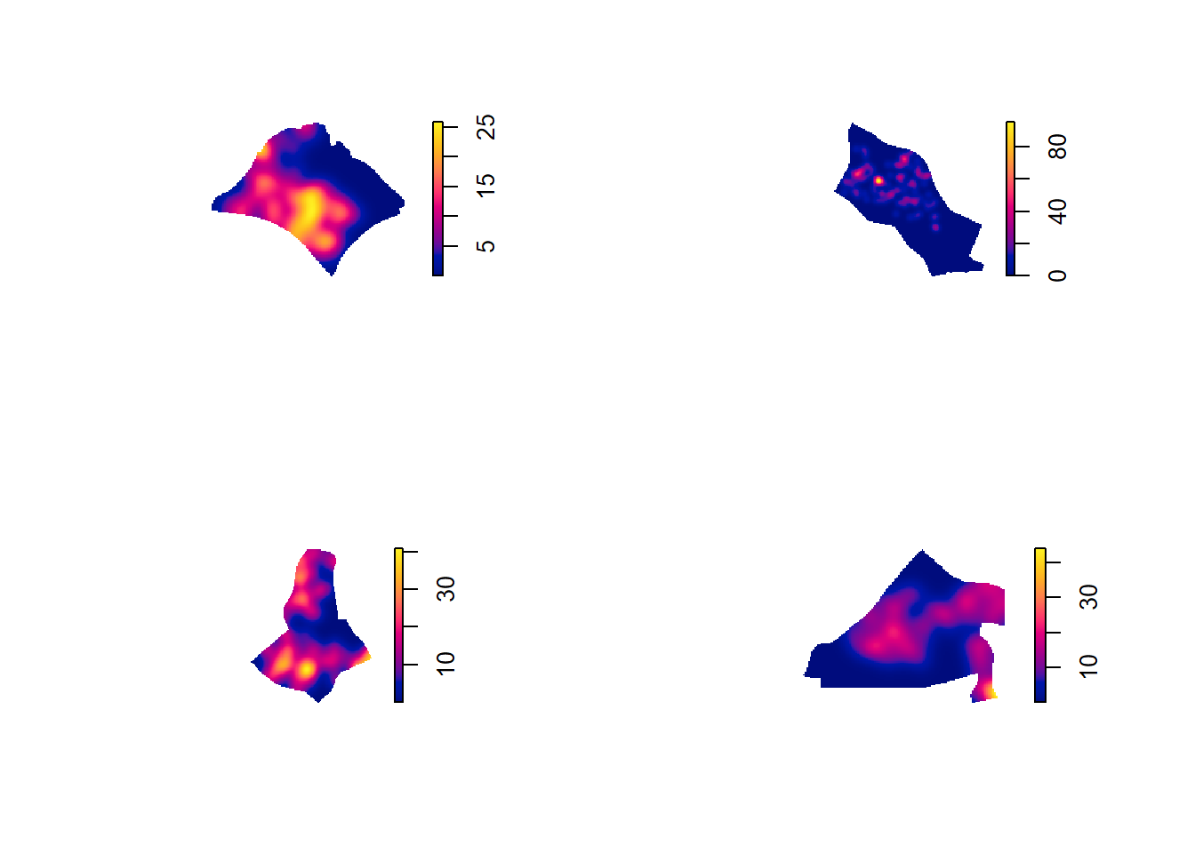
alternative hypothesis: two-sided10.3 Computing KDE surfaces by planning area
The code chunk below will be used to compute the KDE of these four planning area. bw.diggle method is used to derive the bandwidth of each
par(mfrow=c(2,2))
plot(density(childcare_pg_ppp.km,
             sigma=bw.diggle,
             edge=TRUE,
             kernel="gaussian"),
     main="Punggol")
plot(density(childcare_tm_ppp.km,
             sigma=bw.diggle,
             edge=TRUE,
             kernel="gaussian"),
     main="Tempines")
plot(density(childcare_ck_ppp.km,
             sigma=bw.diggle,
             edge=TRUE,
             kernel="gaussian"),
     main="Choa Chu Kang")
plot(density(childcare_jw_ppp.km,
             sigma=bw.diggle,
             edge=TRUE,
             kernel="gaussian"),
     main="Jurong West")