pacman::p_load(sf, terra, spatstat,
tmap, rvest, tidyverse)Hands-on Exercise 2B - Second-order Spatial Point Patterns Analysis Methods
1.Overview
This hands-on exercise explores second-order spatial point pattern analysis to understand how the presence of one childcare centre in Singapore may influence the location of others. Unlike first-order analysis, which focuses on overall density, second-order methods investigate clustering, dispersion, or randomness across spatial scales.
Using functions from the spatstat package in R, the exercise aims to:
Determine whether childcare centres are randomly distributed across Singapore.
If not, identify areas with higher concentrations of centres.
2. Data
Child Care Services data from data.gov.sg, a point feature data providing both location and attribute information of childcare centres.
Master Plan 2019 Subzone Boundary (No Sea), a polygon feature data providing information of URA 2019 Master Plan Planning Subzone boundary data.
3. Installing and Loading the R packages
4. Data Import and Prepration
mpsz_sf <- st_read("data/MasterPlan2019SubzoneBoundaryNoSeaKML (1).kml") %>%
  st_zm(drop = TRUE, what = "ZM") %>% st_transform(crs = 3414)
Reading layer `URA_MP19_SUBZONE_NO_SEA_PL' from data source
`D:\ssinha8752\ISSS608-VAA\Hands-on_Ex\Hands-on_Ex02\data\MasterPlan2019SubzoneBoundaryNoSeaKML (1).kml'
using driver `KML'
Simple feature collection with 332 features and 2 fields
Geometry type: MULTIPOLYGON
Dimension: XY
Bounding box: xmin: 103.6057 ymin: 1.158699 xmax: 104.0885 ymax: 1.470775
Geodetic CRS: WGS 84extract_kml_field <- function(html_text, field_name) {
if (is.na(html_text) || html_text == "") return(NA_character_)
page <- read_html(html_text)
rows <- page %>% html_elements("tr")
value <- rows %>%
keep(~ html_text2(html_element(.x, "th")) == field_name) %>%
html_element("td") %>%
html_text2()
if (length(value) == 0) NA_character_ else value
}mpsz_sf <- mpsz_sf %>%
mutate(
REGION_N = map_chr(Description, extract_kml_field, "REGION_N"),
PLN_AREA_N = map_chr(Description, extract_kml_field, "PLN_AREA_N"),
SUBZONE_N = map_chr(Description, extract_kml_field, "SUBZONE_N"),
SUBZONE_C = map_chr(Description, extract_kml_field, "SUBZONE_C")
) %>%
select(-Name, -Description) %>%
relocate(geometry, .after = last_col())mpsz_cl <- mpsz_sf %>%
filter(SUBZONE_N != "SOUTHERN GROUP",
PLN_AREA_N != "WESTERN ISLANDS",
PLN_AREA_N != "NORTH-EASTERN ISLANDS")write_rds(mpsz_cl, "data/mpsz_cl.rds")childcare_sf <- st_read("data/ChildCareServices.kml") %>%
st_zm(drop = TRUE, what = "ZM") %>%
st_transform(crs = 3414)Reading layer `CHILDCARE' from data source
`D:\ssinha8752\ISSS608-VAA\Hands-on_Ex\Hands-on_Ex02\data\ChildCareServices.kml'
using driver `KML'
Simple feature collection with 1925 features and 2 fields
Geometry type: POINT
Dimension: XYZ
Bounding box: xmin: 103.6878 ymin: 1.247759 xmax: 103.9897 ymax: 1.462134
z_range: zmin: 0 zmax: 0
Geodetic CRS: WGS 84st_crs(mpsz_cl) == st_crs(childcare_sf)[1] TRUElibrary(sf)
library(ggplot2)
library(readr)
# Load cleaned subzone and childcare datasets
mpsz_cl <- read_rds("data/mpsz_cl.rds")
childcare_sf <- st_read("data/ChildCareServices.kml") %>%
st_zm(drop = TRUE, what = "ZM") %>%
st_transform(crs = st_crs(mpsz_cl)) # Ensure same CRSReading layer `CHILDCARE' from data source
`D:\ssinha8752\ISSS608-VAA\Hands-on_Ex\Hands-on_Ex02\data\ChildCareServices.kml'
using driver `KML'
Simple feature collection with 1925 features and 2 fields
Geometry type: POINT
Dimension: XYZ
Bounding box: xmin: 103.6878 ymin: 1.247759 xmax: 103.9897 ymax: 1.462134
z_range: zmin: 0 zmax: 0
Geodetic CRS: WGS 84# Create the map
ggplot() +
geom_sf(data = mpsz_cl, fill = "gray", color = "black", size = 0.2) +
geom_sf(data = childcare_sf, color = "black", size = 1.2, alpha = 0.7) +
labs(title = "Childcare Services Across Singapore Subzones",
subtitle = "All layers aligned to EPSG:3414 (SVY21)",
caption = "Source: URA Master Plan & Data.gov.sg") +
theme_minimal()
Interactive mapping with tmap()
tmap_mode("view")ℹ tmap mode set to "view".tm_shape(childcare_sf) +
tm_dots()Registered S3 method overwritten by 'jsonify':
method from
print.json jsonliteSwitching back to plot
tmap_mode("plot")ℹ tmap mode set to "plot".childcare_ppp <- as.ppp(childcare_sf)class(childcare_ppp)[1] "ppp"summary(childcare_ppp)Marked planar point pattern: 1925 points
Average intensity 2.417323e-06 points per square unit
Coordinates are given to 11 decimal places
Mark variables: Name, Description
Summary:
Name Description
Length:1925 Length:1925
Class :character Class :character
Mode :character Mode :character
Window: rectangle = [11810.03, 45404.24] x [25596.33, 49300.88] units
(33590 x 23700 units)
Window area = 796335000 square unitssg_owin <- as.owin(mpsz_cl)class(sg_owin)[1] "owin"plot(sg_owin)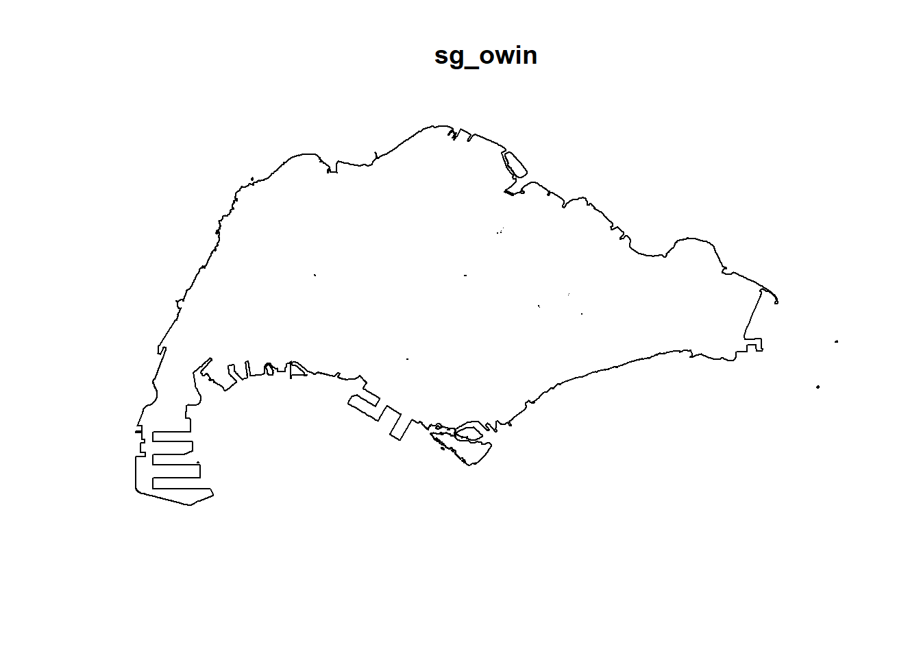
Extraction the childcare events that are located within Singapore by using the code chunk below.
childcareSG_ppp = childcare_ppp[sg_owin]childcareSG_pppMarked planar point pattern: 1925 points
Mark variables: Name, Description
window: polygonal boundary
enclosing rectangle: [2667.54, 55941.94] x [21448.47, 50256.33] unitspg <- mpsz_cl %>%
filter(PLN_AREA_N == "PUNGGOL")
tm <- mpsz_cl %>%
filter(PLN_AREA_N == "TAMPINES")
ck <- mpsz_cl %>%
filter(PLN_AREA_N == "CHOA CHU KANG")
jw <- mpsz_cl %>%
filter(PLN_AREA_N == "JURONG WEST")par(mfrow=c(2,2))
plot(st_geometry(pg), main = "Ponggol")
plot(st_geometry(tm), main = "Tampines")
plot(st_geometry(ck), main = "Choa Chu Kang")
plot(st_geometry(jw), main = "Jurong West")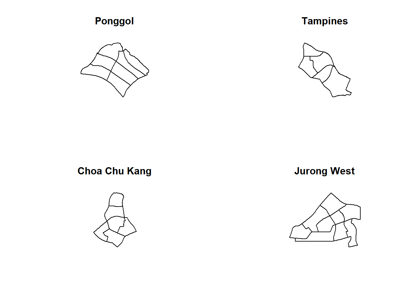
pg_owin = as.owin(pg)
tm_owin = as.owin(tm)
ck_owin = as.owin(ck)
jw_owin = as.owin(jw)
childcare_pg_ppp = childcare_ppp[pg_owin]
childcare_tm_ppp = childcare_ppp[tm_owin]
childcare_ck_ppp = childcare_ppp[ck_owin]
childcare_jw_ppp = childcare_ppp[jw_owin]childcare_pg_ppp.km = rescale.ppp(childcare_pg_ppp, 1000, "km")
childcare_tm_ppp.km = rescale.ppp(childcare_tm_ppp, 1000, "km")
childcare_ck_ppp.km = rescale.ppp(childcare_ck_ppp, 1000, "km")
childcare_jw_ppp.km = rescale.ppp(childcare_jw_ppp, 1000, "km")par(mfrow=c(2,2))
plot(unmark(childcare_pg_ppp.km),
main="Punggol")
plot(unmark(childcare_tm_ppp.km),
main="Tampines")
plot(unmark(childcare_ck_ppp.km),
main="Choa Chu Kang")
plot(unmark(childcare_jw_ppp.km),
main="Jurong West")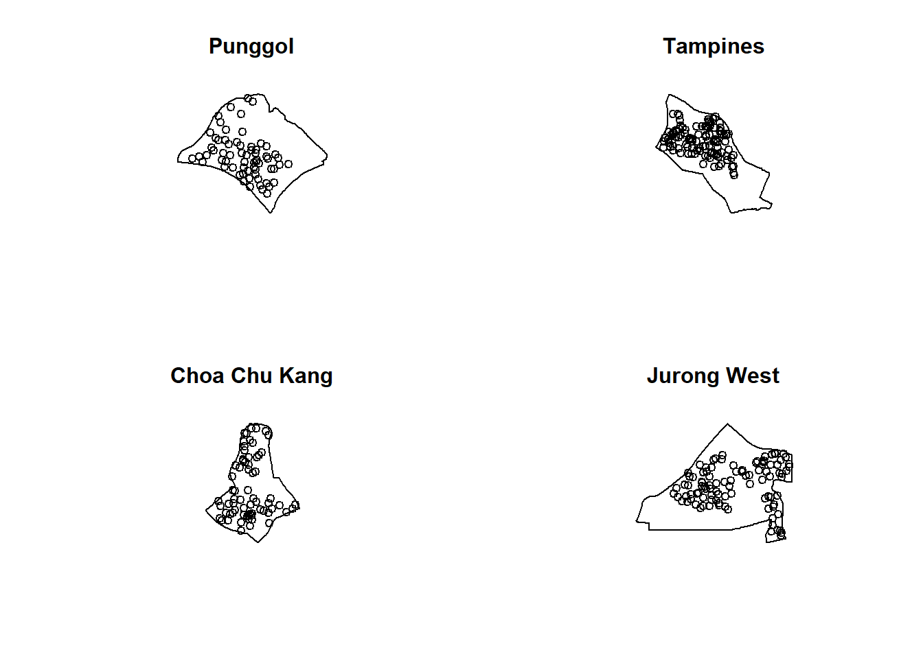
5. Analysing Spatial Point Process Using G-Function
The G function measures the distribution of the distances from an arbitrary event to its nearest event. In this section, you will learn how to compute G-function estimation by using Gest() of spatstat package. You will also learn how to perform monta carlo simulation test using envelope() of spatstat package
5.1 Choa Chu Kang planning area
Computing G-function estimation
set.seed(1234)The code chunk below is used to compute G-function using Gest() of spatat package.
G_CK = Gest(childcare_ck_ppp, correction = "border")
plot(G_CK, xlim=c(0,500))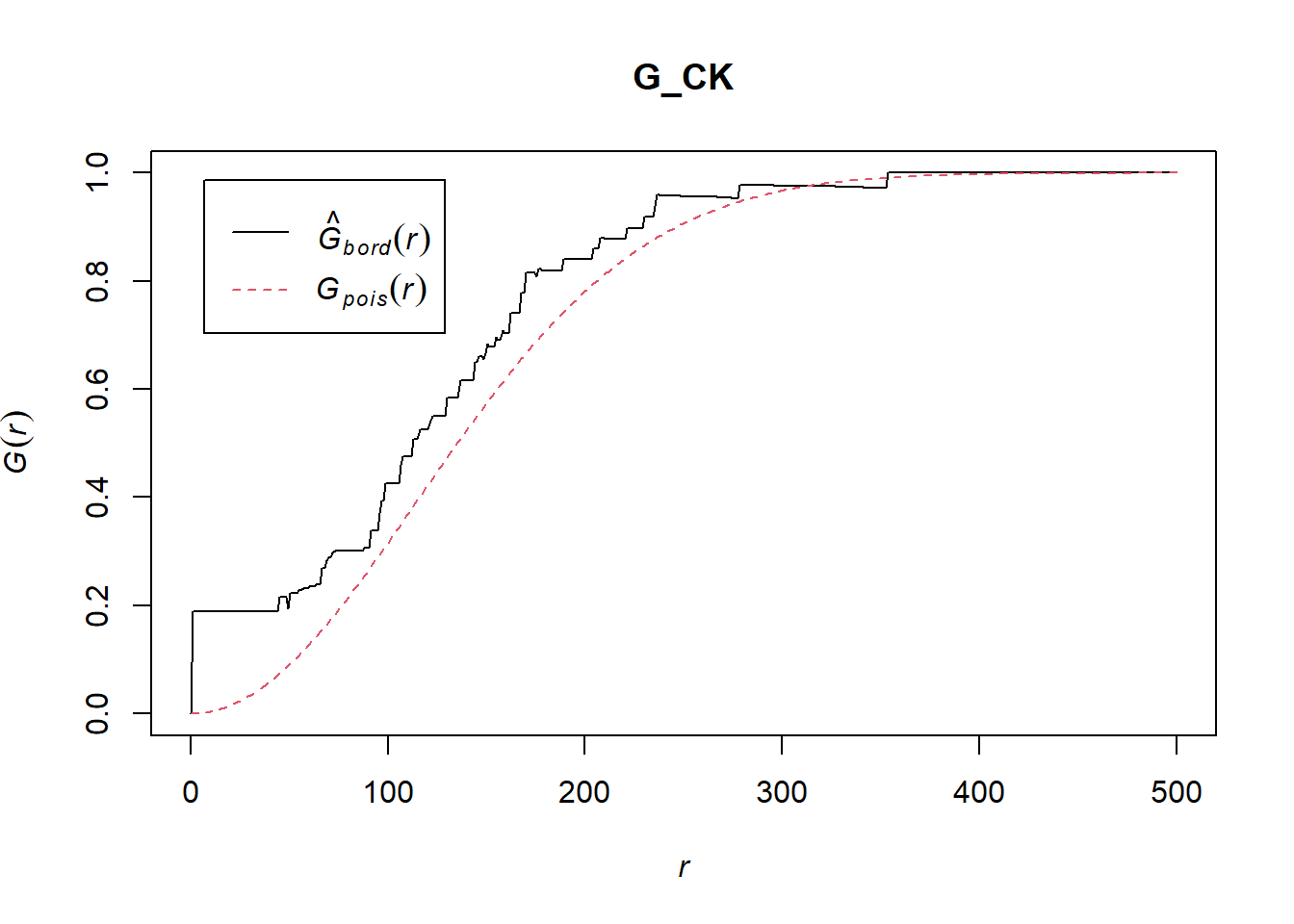
Performing Complete Spatial Randomness Test
To confirm the observed spatial patterns above, a hypothesis test will be conducted. The hypothesis and test are as follows: - Ho = The distribution of childcare services at Choa Chu Kang are randomly distributed. - H1 = The distribution of childcare services at Choa Chu Kang are not randomly distributed.
The null hypothesis will be rejected if p-value is smaller than alpha value of 0.001.
Monte Carlo test with G-fucntion
G_CK.csr <- envelope(childcare_ck_ppp, Gest, nsim = 999)Generating 999 simulations of CSR ...
1, 2, 3, ......10.........20.........30.........40.........50.........60..
.......70.........80.........90.........100.........110.........120.........130
.........140.........150.........160.........170.........180.........190........
.200.........210.........220.........230.........240.........250.........260......
...270.........280.........290.........300.........310.........320.........330....
.....340.........350.........360.........370.........380.........390.........400..
.......410.........420.........430.........440.........450.........460.........470
.........480.........490.........500.........510.........520.........530........
.540.........550.........560.........570.........580.........590.........600......
...610.........620.........630.........640.........650.........660.........670....
.....680.........690.........700.........710.........720.........730.........740..
.......750.........760.........770.........780.........790.........800.........810
.........820.........830.........840.........850.........860.........870........
.880.........890.........900.........910.........920.........930.........940......
...950.........960.........970.........980.........990........
999.
Done.plot(G_CK.csr)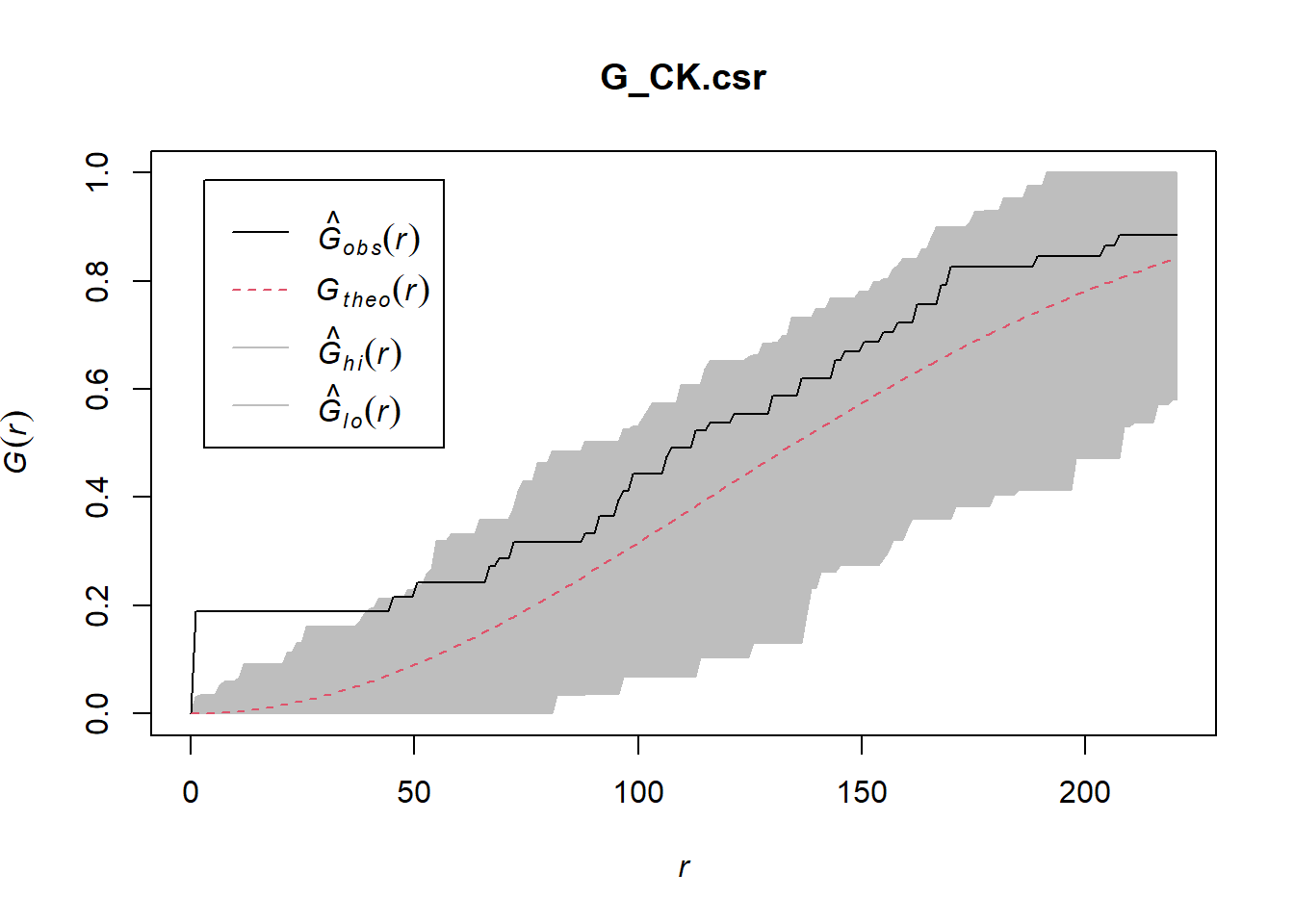
5.2 Tampines planning area
Computing G-function estimation
G_tm = Gest(childcare_tm_ppp, correction = "best")
plot(G_tm)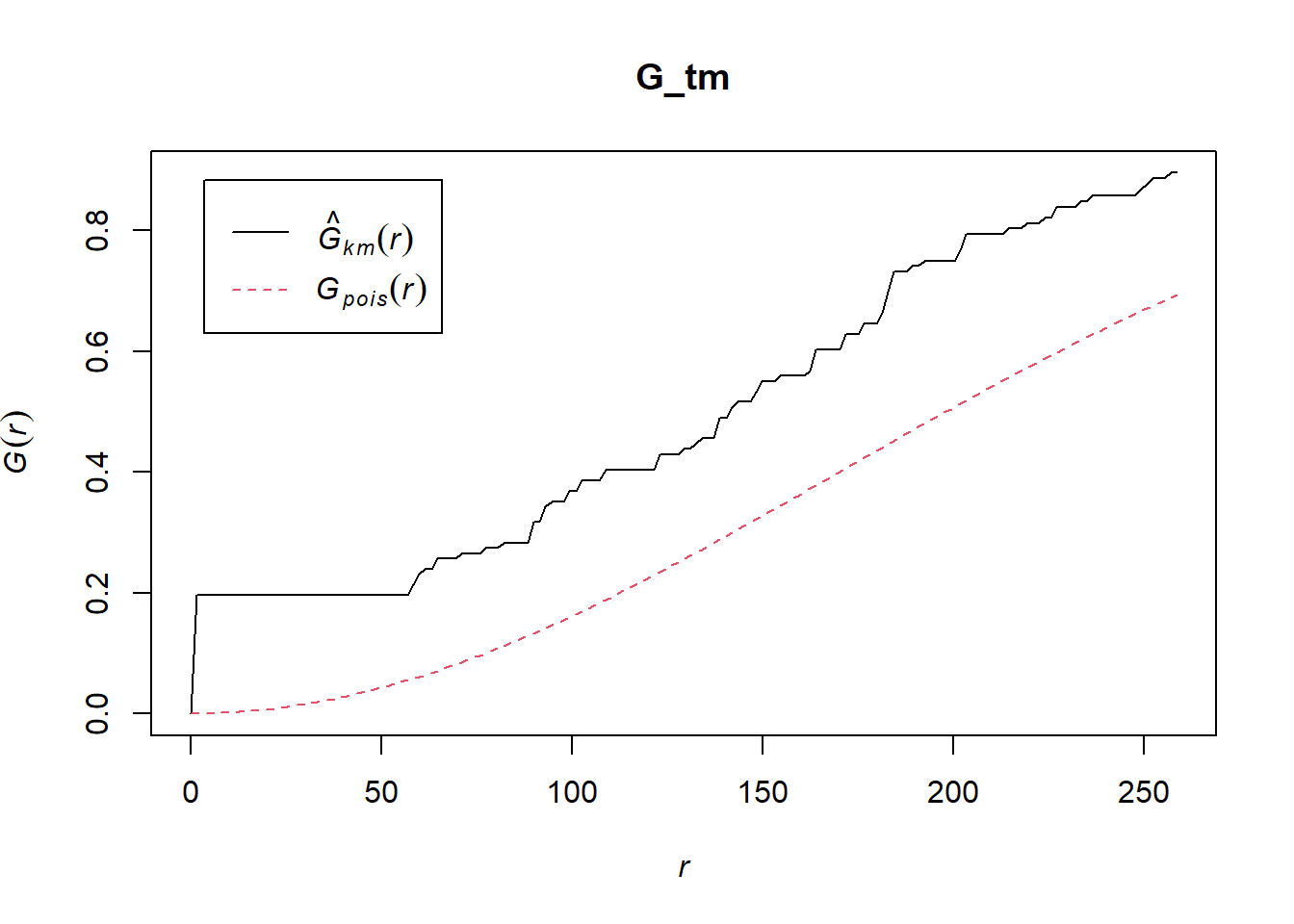
Performing Complete Spatial Randomness Test To confirm the observed spatial patterns above, a hypothesis test will be conducted. The hypothesis and test are as follows: - Ho = The distribution of childcare services at Tampines are randomly distributed. - H1= The distribution of childcare services at Tampines are not randomly distributed.
The null hypothesis will be rejected is p-value is smaller than alpha value of 0.001.
The code chunk below is used to perform the hypothesis testing.
G_tm.csr <- envelope(childcare_tm_ppp, Gest, correction = "all", nsim = 999)Generating 999 simulations of CSR ...
1, 2, 3, ......10.........20.........30.........40.........50.........60..
.......70.........80.........90.........100.........110.........120.........130
.........140.........150.........160.........170.........180.........190........
.200.........210.........220.........230.........240.........250.........260......
...270.........280.........290.........300.........310.........320.........330....
.....340.........350.........360.........370.........380.........390.........400..
.......410.........420.........430.........440.........450.........460.........470
.........480.........490.........500.........510.........520.........530........
.540.........550.........560.........570.........580.........590.........600......
...610.........620.........630.........640.........650.........660.........670....
.....680.........690.........700.........710.........720.........730.........740..
.......750.........760.........770.........780.........790.........800.........810
.........820.........830.........840.........850.........860.........870........
.880.........890.........900.........910.........920.........930.........940......
...950.........960.........970.........980.........990........
999.
Done.plot(G_tm.csr)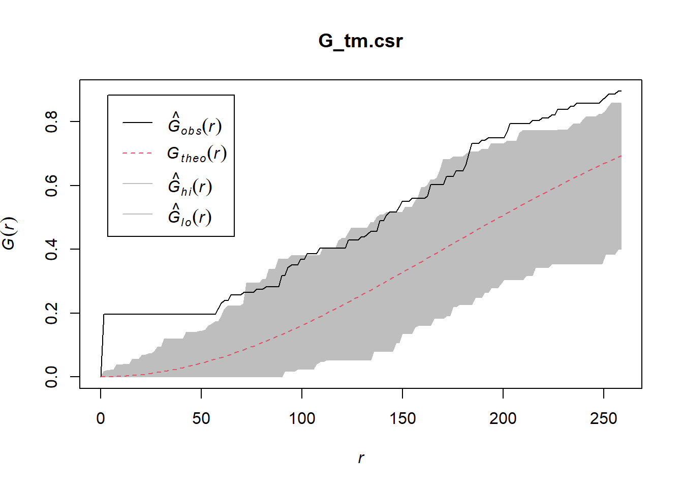
6. Analysing Spatial Point Process Using F-Function
The F function estimates the empty space function F(r) or its hazard rate h(r) from a point pattern in a window of arbitrary shape. In this section, you will learn how to compute F-function estimation by using Fest() of spatstat package. You will also learn how to perform monta carlo simulation test using envelope() of spatstat package.
6.1 Choa Chu Kang planning area
Computing F-function estimation The code chunk below is used to compute F-function using Fest() of spatat package.
F_CK = Fest(childcare_ck_ppp)
plot(F_CK)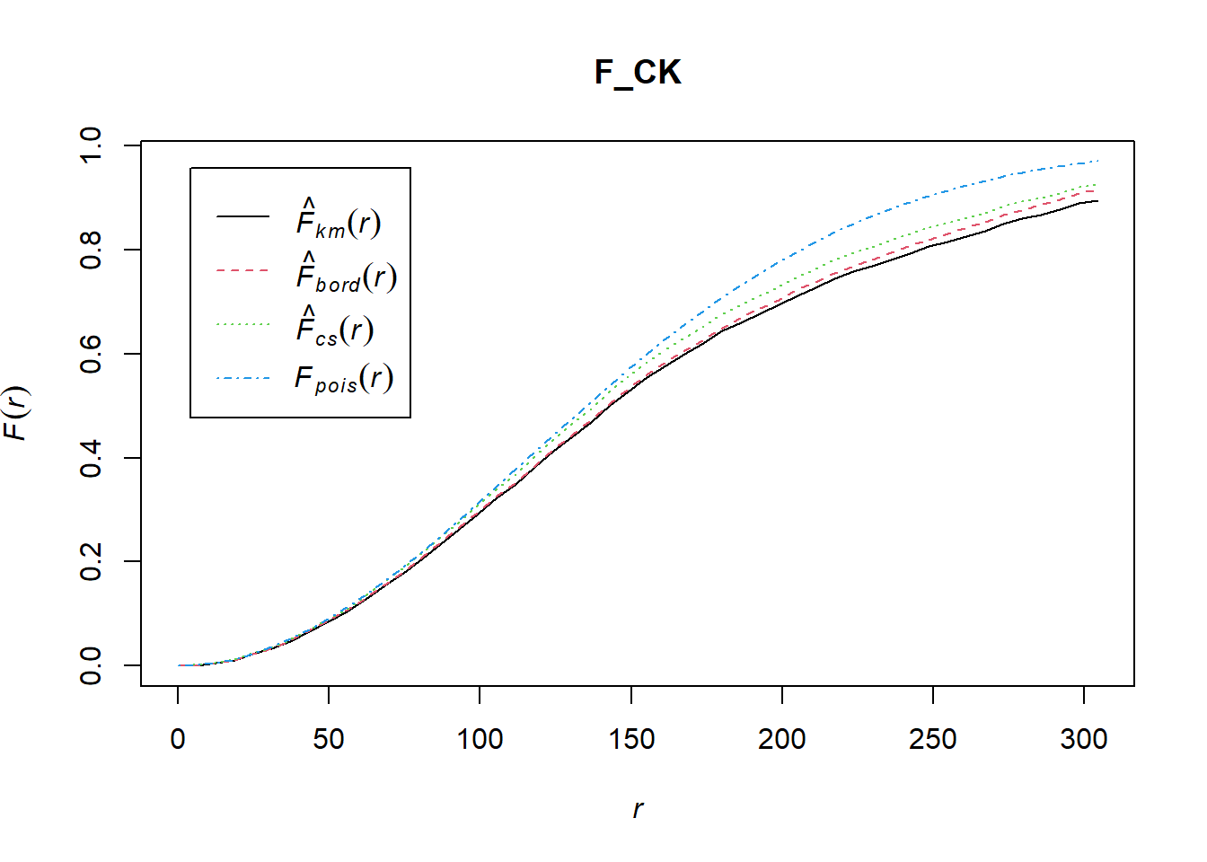
6.2 Performing Complete Spatial Randomness Test
To confirm the observed spatial patterns above, a hypothesis test will be conducted. The hypothesis and test are as follows:
Ho = The distribution of childcare services at Choa Chu Kang are randomly distributed.
H1= The distribution of childcare services at Choa Chu Kang are not randomly distributed.
The null hypothesis will be rejected if p-value is smaller than alpha value of 0.001.
Monte Carlo test with F-fucntion
F_CK.csr <- envelope(childcare_ck_ppp, Fest, nsim = 999)Generating 999 simulations of CSR ...
1, 2, 3, ......10.........20.........30.........40.........50.........60..
.......70.........80.........90.........100.........110.........120.........130
.........140.........150.........160.........170.........180.........190........
.200.........210.........220.........230.........240.........250.........260......
...270.........280.........290.........300.........310.........320.........330....
.....340.........350.........360.........370.........380.........390.........400..
.......410.........420.........430.........440.........450.........460.........470
.........480.........490.........500.........510.........520.........530........
.540.........550.........560.........570.........580.........590.........600......
...610.........620.........630.........640.........650.........660.........670....
.....680.........690.........700.........710.........720.........730.........740..
.......750.........760.........770.........780.........790.........800.........810
.........820.........830.........840.........850.........860.........870........
.880.........890.........900.........910.........920.........930.........940......
...950.........960.........970.........980.........990........
999.
Done.plot(F_CK.csr)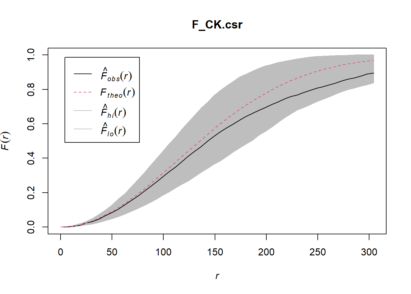
6.3 Tampines planning area
Computing F-function estimation Monte Carlo test with F-fucntion
F_tm = Fest(childcare_tm_ppp, correction = "best")
plot(F_tm)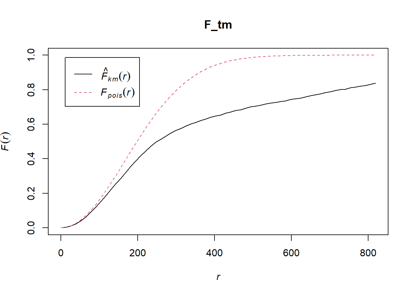
Performing Complete Spatial Randomness Test To confirm the observed spatial patterns above, a hypothesis test will be conducted. The hypothesis and test are as follows:
Ho = The distribution of childcare services at Tampines are randomly distributed.
H1= The distribution of childcare services at Tampines are not randomly distributed.
The null hypothesis will be rejected is p-value is smaller than alpha value of 0.001.
The code chunk below is used to perform the hypothesis testing.
F_tm.csr <- envelope(childcare_tm_ppp, Fest, correction = "all", nsim = 999)Generating 999 simulations of CSR ...
1, 2, 3, ......10.........20.........30.........40.........50.........60..
.......70.........80.........90.........100.........110.........120.........130
.........140.........150.........160.........170.........180.........190........
.200.........210.........220.........230.........240.........250.........260......
...270.........280.........290.........300.........310.........320.........330....
.....340.........350.........360.........370.........380.........390.........400..
.......410.........420.........430.........440.........450.........460.........470
.........480.........490.........500.........510.........520.........530........
.540.........550.........560.........570.........580.........590.........600......
...610.........620.........630.........640.........650.........660.........670....
.....680.........690.........700.........710.........720.........730.........740..
.......750.........760.........770.........780.........790.........800.........810
.........820.........830.........840.........850.........860.........870........
.880.........890.........900.........910.........920.........930.........940......
...950.........960.........970.........980.........990........
999.
Done.plot(F_tm.csr)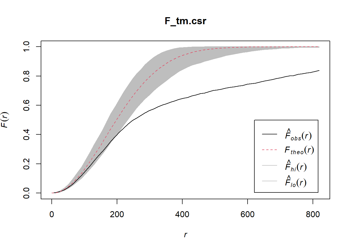
7. Analysing Spatial Point Process Using K-Function
K-function measures the number of events found up to a given distance of any particular event. In this section, you will learn how to compute K-function estimates by using Kest() of spatstat package. You will also learn how to perform monta carlo simulation test using envelope() of spatstat package.
7.1 Choa Chu Kang planning area
Computing K-fucntion estimate
K_ck = Kest(childcare_ck_ppp, correction = "Ripley")
plot(K_ck, . -r ~ r, ylab= "K(d)-r", xlab = "d(m)")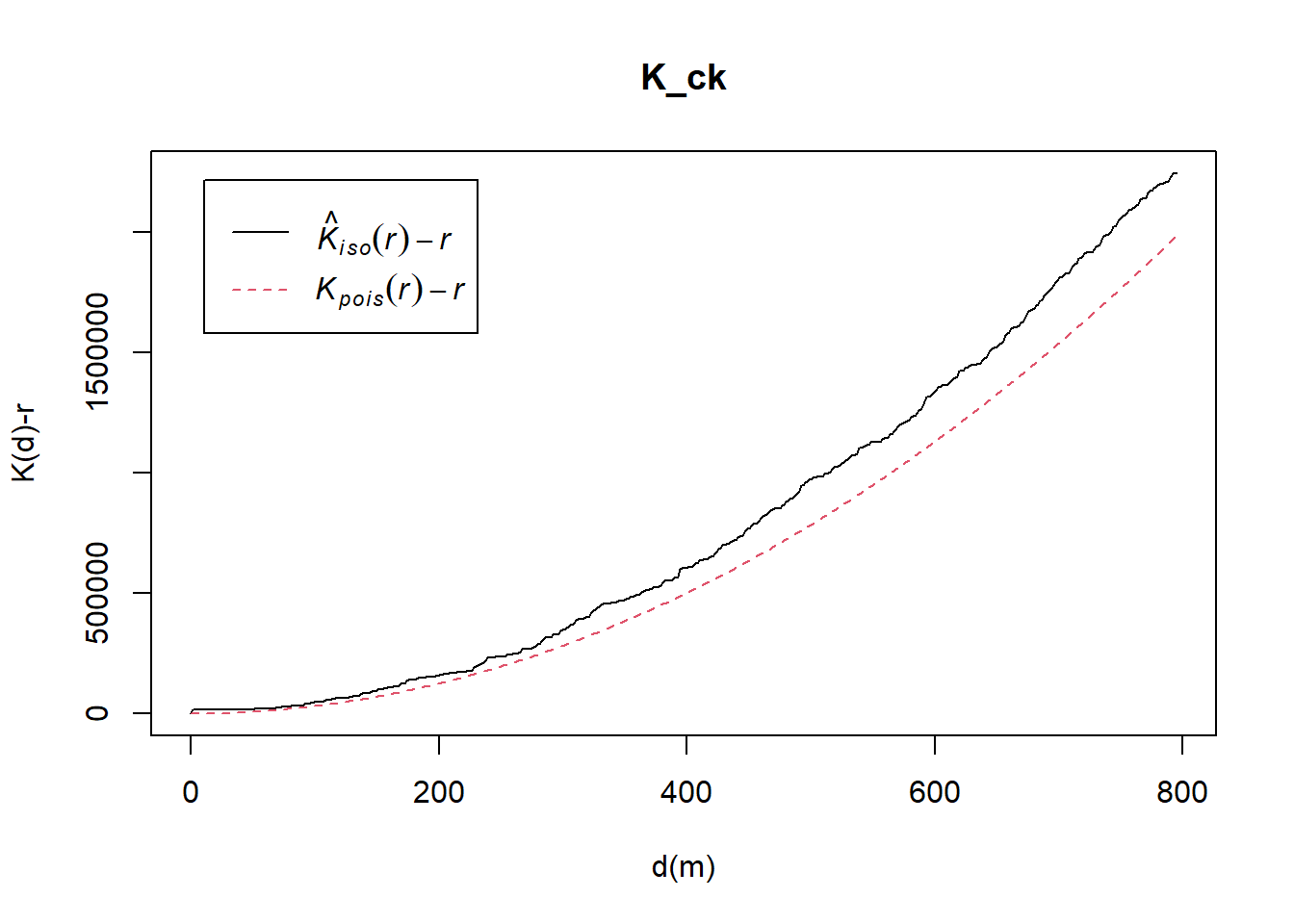
Performing Complete Spatial Randomness Test To confirm the observed spatial patterns above, a hypothesis test will be conducted. The hypothesis and test are as follows:
Ho = The distribution of childcare services at Choa Chu Kang are randomly distributed.
H1= The distribution of childcare services at Choa Chu Kang are not randomly distributed.
The null hypothesis will be rejected if p-value is smaller than alpha value of 0.001.
The code chunk below is used to perform the hypothesis testing.
K_ck.csr <- envelope(childcare_ck_ppp, Kest, nsim = 99, rank = 1, glocal=TRUE)Generating 99 simulations of CSR ...
1, 2, 3, 4, 5, 6, 7, 8, 9, 10, 11, 12, 13, 14, 15, 16, 17, 18, 19, 20,
21, 22, 23, 24, 25, 26, 27, 28, 29, 30, 31, 32, 33, 34, 35, 36, 37, 38, 39, 40,
41, 42, 43, 44, 45, 46, 47, 48, 49, 50, 51, 52, 53, 54, 55, 56, 57, 58, 59, 60,
61, 62, 63, 64, 65, 66, 67, 68, 69, 70, 71, 72, 73, 74, 75, 76, 77, 78, 79, 80,
81, 82, 83, 84, 85, 86, 87, 88, 89, 90, 91, 92, 93, 94, 95, 96, 97, 98,
99.
Done.plot(K_ck.csr, . - r ~ r, xlab="d", ylab="K(d)-r")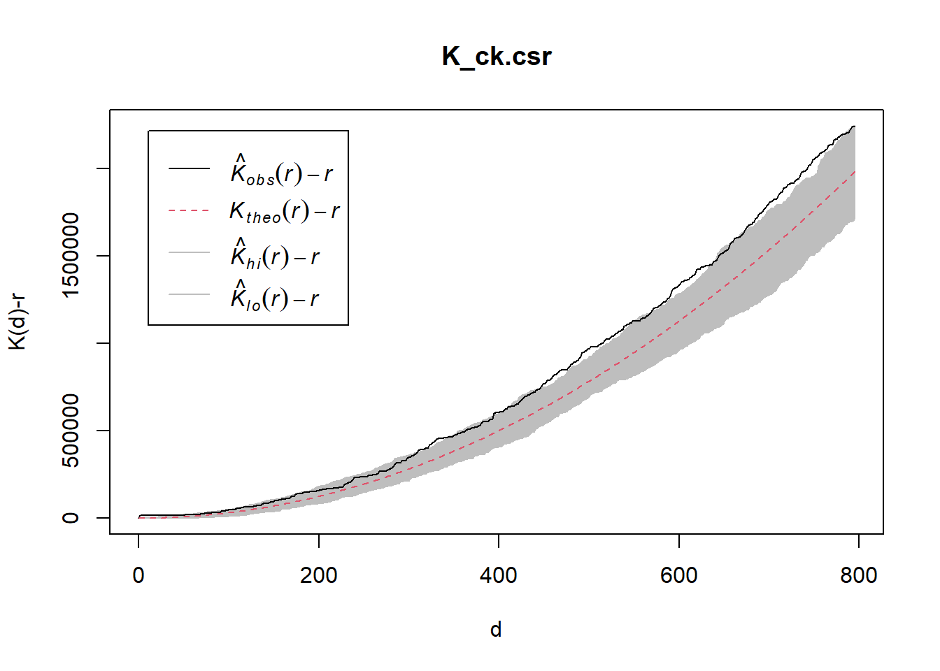
7.2 Tampines planning area
Computing K-fucntion estimation
K_tm = Kest(childcare_tm_ppp, correction = "Ripley")
plot(K_tm, . -r ~ r,
     ylab= "K(d)-r", xlab = "d(m)",
     xlim=c(0,1000))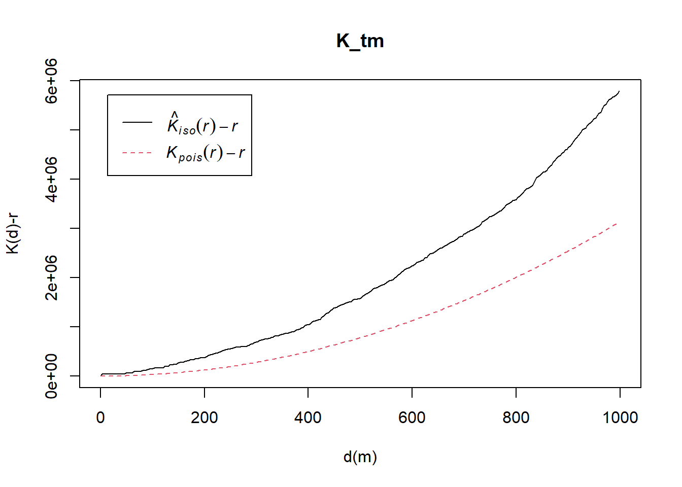
Performing Complete Spatial Randomness Test To confirm the observed spatial patterns above, a hypothesis test will be conducted. The hypothesis and test are as follows:
Ho = The distribution of childcare services at Tampines are randomly distributed.
H1= The distribution of childcare services at Tampines are not randomly distributed.
The null hypothesis will be rejected if p-value is smaller than alpha value of 0.001.
The code chunk below is used to perform the hypothesis testing.
K_tm.csr <- envelope(childcare_tm_ppp, Kest, nsim = 99, rank = 1, glocal=TRUE)Generating 99 simulations of CSR ...
1, 2, 3, 4, 5, 6, 7, 8, 9, 10, 11, 12, 13, 14, 15, 16, 17, 18, 19, 20,
21, 22, 23, 24, 25, 26, 27, 28, 29, 30, 31, 32, 33, 34, 35, 36, 37, 38, 39, 40,
41, 42, 43, 44, 45, 46, 47, 48, 49, 50, 51, 52, 53, 54, 55, 56, 57, 58, 59, 60,
61, 62, 63, 64, 65, 66, 67, 68, 69, 70, 71, 72, 73, 74, 75, 76, 77, 78, 79, 80,
81, 82, 83, 84, 85, 86, 87, 88, 89, 90, 91, 92, 93, 94, 95, 96, 97, 98,
99.
Done.plot(K_tm.csr, . - r ~ r,
xlab="d", ylab="K(d)-r", xlim=c(0,500))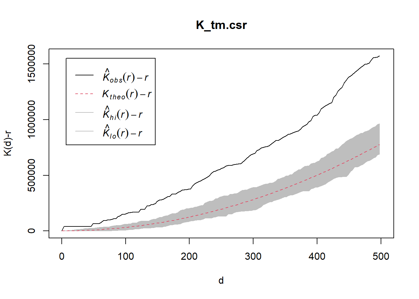
8.Analysing Spatial Point Process Using L-Function
how to compute L-function estimation by using Lest() of spatstat package. And will also learn how to perform monta carlo simulation test using envelope() of spatstat package.
8.1 Choa Chu Kang planning area
Computing L Fucntion estimation
L_ck = Lest(childcare_ck_ppp, correction = "Ripley")
plot(L_ck, . -r ~ r,
     ylab= "L(d)-r", xlab = "d(m)")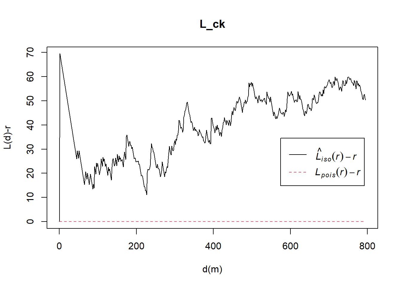
Performing Complete Spatial Randomness Test To confirm the observed spatial patterns above, a hypothesis test will be conducted. The hypothesis and test are as follows:
Ho = The distribution of childcare services at Choa Chu Kang are randomly distributed.
H1= The distribution of childcare services at Choa Chu Kang are not randomly distributed.
The null hypothesis will be rejected if p-value if smaller than alpha value of 0.001.
The code chunk below is used to perform the hypothesis testing.
L_ck.csr <- envelope(childcare_ck_ppp, Lest, nsim = 99, rank = 1, glocal=TRUE)Generating 99 simulations of CSR ...
1, 2, 3, 4, 5, 6, 7, 8, 9, 10, 11, 12, 13, 14, 15, 16, 17, 18, 19, 20,
21, 22, 23, 24, 25, 26, 27, 28, 29, 30, 31, 32, 33, 34, 35, 36, 37, 38, 39, 40,
41, 42, 43, 44, 45, 46, 47, 48, 49, 50, 51, 52, 53, 54, 55, 56, 57, 58, 59, 60,
61, 62, 63, 64, 65, 66, 67, 68, 69, 70, 71, 72, 73, 74, 75, 76, 77, 78, 79, 80,
81, 82, 83, 84, 85, 86, 87, 88, 89, 90, 91, 92, 93, 94, 95, 96, 97, 98,
99.
Done.plot(L_ck.csr, . - r ~ r, xlab="d", ylab="L(d)-r")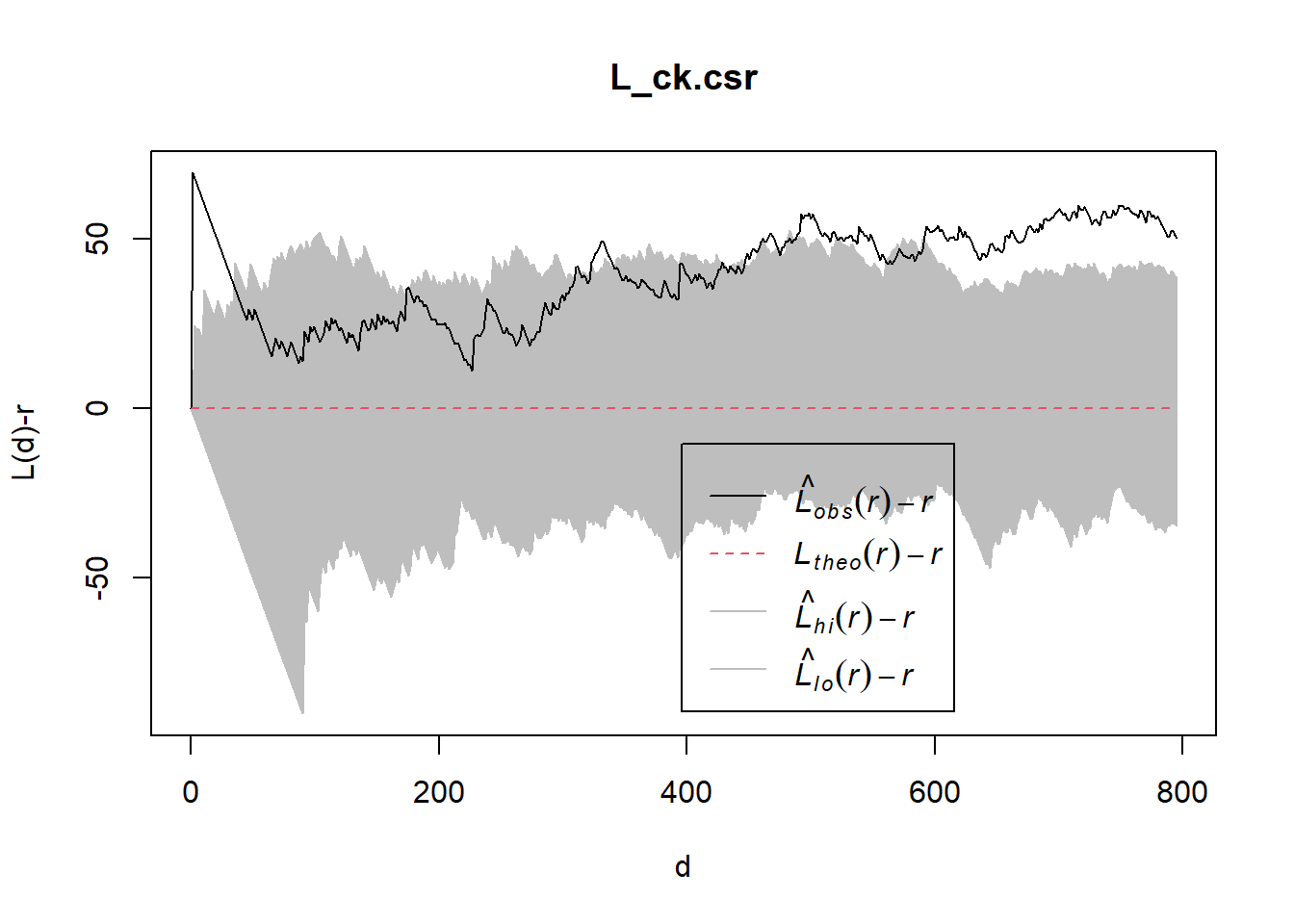
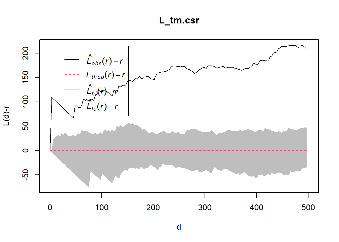
8.2 Tampines planning area
Computing L-fucntion estimate
L_tm = Lest(childcare_tm_ppp, correction = "Ripley")
plot(L_tm, . -r ~ r,
     ylab= "L(d)-r", xlab = "d(m)",
     xlim=c(0,1000))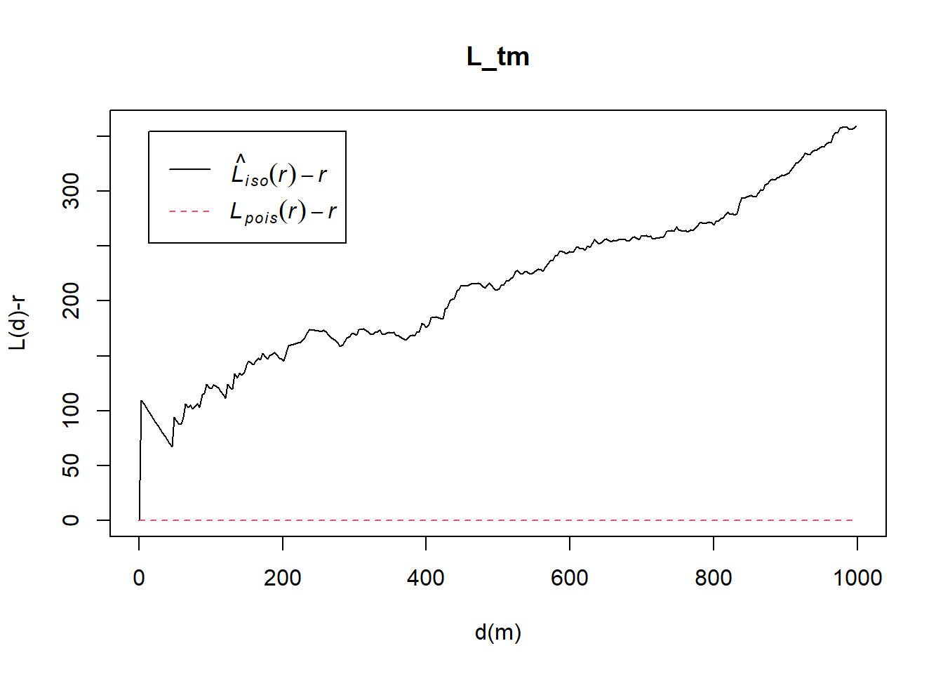
Performing Complete Spatial Randomness Test To confirm the observed spatial patterns above, a hypothesis test will be conducted. The hypothesis and test are as follows:
Ho = The distribution of childcare services at Tampines are randomly distributed.
H1= The distribution of childcare services at Tampines are not randomly distributed.
The null hypothesis will be rejected if p-value is smaller than alpha value of 0.001.
The code chunk below will be used to perform the hypothesis testing.
L_tm.csr <- envelope(childcare_tm_ppp, Lest, nsim = 99, rank = 1, glocal=TRUE)Generating 99 simulations of CSR ...
1, 2, 3, 4, 5, 6, 7, 8, 9, 10, 11, 12, 13, 14, 15, 16, 17, 18, 19, 20,
21, 22, 23, 24, 25, 26, 27, 28, 29, 30, 31, 32, 33, 34, 35, 36, 37, 38, 39, 40,
41, 42, 43, 44, 45, 46, 47, 48, 49, 50, 51, 52, 53, 54, 55, 56, 57, 58, 59, 60,
61, 62, 63, 64, 65, 66, 67, 68, 69, 70, 71, 72, 73, 74, 75, 76, 77, 78, 79, 80,
81, 82, 83, 84, 85, 86, 87, 88, 89, 90, 91, 92, 93, 94, 95, 96, 97, 98,
99.
Done.plot(L_tm.csr, . - r ~ r,
xlab="d", ylab="L(d)-r", xlim=c(0,500))