In-class Exercise 3b : Working with Open Government Data

1 Load the R package

pacman::p_load(sf, tmap, tidyverse,httr)

2 Import the ACRA data

folder_path <- "data/aspatial/ACRA"
file_list <- list.files(path = folder_path,
                        pattern = "^ACRA*.*\\.csv$",
                        full.names = TRUE)

acra_data <- file_list %>%
  map_dfr(read_csv)

3 Saving the ACRA data

write_rds(acra_data,
          "data/rds/acra_data.rds")

4 Tidying the ACRA data

biz_56111 <- acra_data %>%
  select(1:24) %>%
  filter(primary_ssic_code == 56111) %>%
  rename(date = registration_incorporation_date) %>%
  mutate(date = as.Date(date),
         YEAR = year(date),
         MONTH_NUM = month(date),
         MONTH_ABBR = month(date,
                            label = TRUE,
                            abbr = TRUE)) %>%
  mutate(
    postal_code = str_pad(postal_code,
    width = 6, side = "left", pad = "0")) %>%
            filter(YEAR == 2025)

5 Geocoding

postcodes <- unique(biz_56111$postal_code)

url <- "https://onemap.gov.sg/api/common/elastic/search"


found <-data.frame()
not_found <- data.frame(postcode = character())

for(pc in postcodes) {
  query <- list(
    searchVal = pc,
    returnGeom = "Y",
    getAddrDetails = "Y",
    pageNum = "1"
  )
  
  res <- GET(url,query = query)
  json <- content(res)
  
  if(json$found !=0) {
    df <- as.data.frame(json$results,stringAsFactors = FALSE)
    df$input_postcode <- pc
    found <- bind_rows(found,df)
  } else {
    not_found <- bind_rows(not_found,data,frame(postcode = pc))
  }
}

6 Tidying the geocoded data

found <- found %>%
  select(1:10)

7 Appending the location information

biz_56111 = biz_56111 %>%
  left_join(found,
            by = c('postal_code' = 'POSTAL'))

8 Saving the data

write_rds(biz_56111, "data/rds/biz_56111.rds")

9 Converting into SF data frame

biz_56111_sf <- st_as_sf(biz_56111, 
                         coords = c("X", "Y"),
                         crs = 3414)

10 Visualization of the distribution

ggplot(data = biz_56111,
       aes(x = MONTH_ABBR)) +
  geom_bar()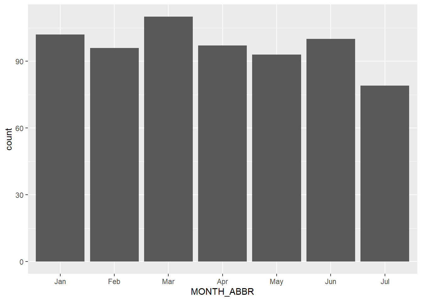

11 Visualizaing the business

tmap_mode('view')
tm_shape(biz_56111_sf)+
  tm_dots()