In-class Exercise 2: Spatial Point Patterns Analysis

Author

Shubham Sinha

Published

September 6, 2025

Modified

September 13, 2025

1 Installing and loading R packages

1.1 Install maptools package

maptools is retired and its binary is removed from CRAN. However, we can download it from Posit Public Package Manager snapshots by using following code

code chunk

install.packages("maptools",
                 repos = "https://packagemanager.posit.co/cran/2023-10-13")

Include #| eval: false in the code chunk to avoid maptools being downloaded and installed repetitively every time the Quarto document is rendered.

1.2 Install remaining packages

The code chunk below install and load following packages into R environment:

sf, a relatively new R package specially designed to import, manage and process vector-based geospatial data in R.
spatstat, which has a wide range of useful functions for point pattern analysis. In this hands-on exercise, it will be used to perform 1st- and 2nd-order spatial point patterns analysis and derive kernel density estimation (KDE) layer.
raster which reads, writes, manipulates, analyses and model of gridded spatial data (i.e. raster). In this hands-on exercise, it will be used to convert image output generate by spatstat into raster format.
maptools which provides a set of tools for manipulating geographic data. In this hands-on exercise, we mainly use it to convert Spatial objects into ppp format of spatstat.
tmap which provides functions for plotting cartographic quality static point patterns maps or interactive maps by using leaflet API.

code chunk

pacman::p_load(sf, raster, spatstat, tmap, tidyverse)

2 The data

Data sets in this exercise are as follows:

CHILDCARE (Point Feature Data)
- This dataset provides both location and attribute information of childcare centres across Singapore.
- Format: GeoJSON
- Source: data.gov.sg
MP14_SUBZONE_WEB_PL (Polygon Feature Data)
- This dataset provide information of URA 2014 Master Plan Planning Subzone boundary data.
- Format: ESRI Shapefile.
- Source: data.gov.sg
CostalOutline (Polygon Feature Data)
- This dataset shows the national boundary of Singapore.
- Format: ESRI Shapefile
- Source: Singapore Land Authority

We will use st_read() of sf package will be used to import these three geospatial data sets into R.

Childcare data
Master Plan 2014 data

Since the childcare_sf simple feature data frame is in the WGS84 geodetic CRS, which is not ideal for geospatial analysis, the st_transform() function from the sf package is used to reproject the data to the SVY21 coordinate system during import.

code chunk

childcare_sf <- st_read("data/ChildCareServices.geojson") %>%
  st_transform(crs = 3414)

Reading layer `ChildCareServices' from data source 
  `D:\ssinha8752\ISSS608-VAA\In-class_Ex\In-class_Ex02\data\ChildCareServices.geojson' 
  using driver `GeoJSON'
Simple feature collection with 1925 features and 2 fields
Geometry type: POINT
Dimension:     XYZ
Bounding box:  xmin: 103.6878 ymin: 1.247759 xmax: 103.9897 ymax: 1.462134
z_range:       zmin: 0 zmax: 0
Geodetic CRS:  WGS 84

Let’s verify the crs of the data frame to ensure we’re using EPSG 3414.

code chunk

st_crs(childcare_sf)

Coordinate Reference System:
  User input: EPSG:3414 
  wkt:
PROJCRS["SVY21 / Singapore TM",
    BASEGEOGCRS["SVY21",
        DATUM["SVY21",
            ELLIPSOID["WGS 84",6378137,298.257223563,
                LENGTHUNIT["metre",1]]],
        PRIMEM["Greenwich",0,
            ANGLEUNIT["degree",0.0174532925199433]],
        ID["EPSG",4757]],
    CONVERSION["Singapore Transverse Mercator",
        METHOD["Transverse Mercator",
            ID["EPSG",9807]],
        PARAMETER["Latitude of natural origin",1.36666666666667,
            ANGLEUNIT["degree",0.0174532925199433],
            ID["EPSG",8801]],
        PARAMETER["Longitude of natural origin",103.833333333333,
            ANGLEUNIT["degree",0.0174532925199433],
            ID["EPSG",8802]],
        PARAMETER["Scale factor at natural origin",1,
            SCALEUNIT["unity",1],
            ID["EPSG",8805]],
        PARAMETER["False easting",28001.642,
            LENGTHUNIT["metre",1],
            ID["EPSG",8806]],
        PARAMETER["False northing",38744.572,
            LENGTHUNIT["metre",1],
            ID["EPSG",8807]]],
    CS[Cartesian,2],
        AXIS["northing (N)",north,
            ORDER[1],
            LENGTHUNIT["metre",1]],
        AXIS["easting (E)",east,
            ORDER[2],
            LENGTHUNIT["metre",1]],
    USAGE[
        SCOPE["Cadastre, engineering survey, topographic mapping."],
        AREA["Singapore - onshore and offshore."],
        BBOX[1.13,103.59,1.47,104.07]],
    ID["EPSG",3414]]

Let’s load the Master Plan Planning data using st_read() function

code chunk

mpsz_sf <- st_read(dsn = "data", 
                layer = "MP14_SUBZONE_WEB_PL")

Reading layer `MP14_SUBZONE_WEB_PL' from data source 
  `D:\ssinha8752\ISSS608-VAA\In-class_Ex\In-class_Ex02\data' 
  using driver `ESRI Shapefile'
Simple feature collection with 323 features and 15 fields
Geometry type: MULTIPOLYGON
Dimension:     XY
Bounding box:  xmin: 2667.538 ymin: 15748.72 xmax: 56396.44 ymax: 50256.33
Projected CRS: SVY21

Let’s check coordinate system of this data frame

code chunk

st_crs(mpsz_sf)

Coordinate Reference System:
  User input: SVY21 
  wkt:
PROJCRS["SVY21",
    BASEGEOGCRS["SVY21[WGS84]",
        DATUM["World Geodetic System 1984",
            ELLIPSOID["WGS 84",6378137,298.257223563,
                LENGTHUNIT["metre",1]],
            ID["EPSG",6326]],
        PRIMEM["Greenwich",0,
            ANGLEUNIT["Degree",0.0174532925199433]]],
    CONVERSION["unnamed",
        METHOD["Transverse Mercator",
            ID["EPSG",9807]],
        PARAMETER["Latitude of natural origin",1.36666666666667,
            ANGLEUNIT["Degree",0.0174532925199433],
            ID["EPSG",8801]],
        PARAMETER["Longitude of natural origin",103.833333333333,
            ANGLEUNIT["Degree",0.0174532925199433],
            ID["EPSG",8802]],
        PARAMETER["Scale factor at natural origin",1,
            SCALEUNIT["unity",1],
            ID["EPSG",8805]],
        PARAMETER["False easting",28001.642,
            LENGTHUNIT["metre",1],
            ID["EPSG",8806]],
        PARAMETER["False northing",38744.572,
            LENGTHUNIT["metre",1],
            ID["EPSG",8807]]],
    CS[Cartesian,2],
        AXIS["(E)",east,
            ORDER[1],
            LENGTHUNIT["metre",1,
                ID["EPSG",9001]]],
        AXIS["(N)",north,
            ORDER[2],
            LENGTHUNIT["metre",1,
                ID["EPSG",9001]]]]

mpsz_sf is also using EPSG 9001 instead of 3414 which is suitable for CRS SVY21. Let’s assign correct EPSG code using st_set_crs() then verify the output.

code chunk

mpsz_sf <- st_set_crs(mpsz_sf,3414)

Warning: st_crs<- : replacing crs does not reproject data; use st_transform for
that

code chunk

st_crs(mpsz_sf)

Coordinate Reference System:
  User input: EPSG:3414 
  wkt:
PROJCRS["SVY21 / Singapore TM",
    BASEGEOGCRS["SVY21",
        DATUM["SVY21",
            ELLIPSOID["WGS 84",6378137,298.257223563,
                LENGTHUNIT["metre",1]]],
        PRIMEM["Greenwich",0,
            ANGLEUNIT["degree",0.0174532925199433]],
        ID["EPSG",4757]],
    CONVERSION["Singapore Transverse Mercator",
        METHOD["Transverse Mercator",
            ID["EPSG",9807]],
        PARAMETER["Latitude of natural origin",1.36666666666667,
            ANGLEUNIT["degree",0.0174532925199433],
            ID["EPSG",8801]],
        PARAMETER["Longitude of natural origin",103.833333333333,
            ANGLEUNIT["degree",0.0174532925199433],
            ID["EPSG",8802]],
        PARAMETER["Scale factor at natural origin",1,
            SCALEUNIT["unity",1],
            ID["EPSG",8805]],
        PARAMETER["False easting",28001.642,
            LENGTHUNIT["metre",1],
            ID["EPSG",8806]],
        PARAMETER["False northing",38744.572,
            LENGTHUNIT["metre",1],
            ID["EPSG",8807]]],
    CS[Cartesian,2],
        AXIS["northing (N)",north,
            ORDER[1],
            LENGTHUNIT["metre",1]],
        AXIS["easting (E)",east,
            ORDER[2],
            LENGTHUNIT["metre",1]],
    USAGE[
        SCOPE["Cadastre, engineering survey, topographic mapping."],
        AREA["Singapore - onshore and offshore."],
        BBOX[1.13,103.59,1.47,104.07]],
    ID["EPSG",3414]]

2.1 working with `st_union()`

is used to derive the coastal outline sf tibble data.frame

code chunk

sg_sf <- mpsz_sf %>%
  st_union()

sg_sf will look similar to the figure below.

code chunk

plot(sg_sf)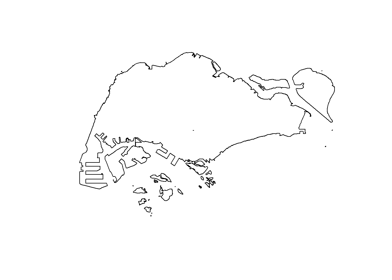

3 Creating ppp objects from sf data.frame

We can use as.ppp() of spatstat.geom package to derive an ppp object layer directly from a sf tibble data.frame.

code chunk

# Check geometry
print(st_geometry(childcare_sf))

Geometry set for 1925 features 
Geometry type: POINT
Dimension:     XYZ
Bounding box:  xmin: 11810.03 ymin: 25596.33 xmax: 45404.24 ymax: 49300.88
z_range:       zmin: 0 zmax: 0
Projected CRS: SVY21 / Singapore TM
First 5 geometries:

POINT Z (40985.94 33848.38 0)

POINT Z (28308.65 45530.47 0)

POINT Z (17828.84 36607.36 0)

POINT Z (25579.73 29221.89 0)

POINT Z (38981.02 32483.41 0)

code chunk

# Check CRS
print(st_crs(childcare_sf))

Coordinate Reference System:
  User input: EPSG:3414 
  wkt:
PROJCRS["SVY21 / Singapore TM",
    BASEGEOGCRS["SVY21",
        DATUM["SVY21",
            ELLIPSOID["WGS 84",6378137,298.257223563,
                LENGTHUNIT["metre",1]]],
        PRIMEM["Greenwich",0,
            ANGLEUNIT["degree",0.0174532925199433]],
        ID["EPSG",4757]],
    CONVERSION["Singapore Transverse Mercator",
        METHOD["Transverse Mercator",
            ID["EPSG",9807]],
        PARAMETER["Latitude of natural origin",1.36666666666667,
            ANGLEUNIT["degree",0.0174532925199433],
            ID["EPSG",8801]],
        PARAMETER["Longitude of natural origin",103.833333333333,
            ANGLEUNIT["degree",0.0174532925199433],
            ID["EPSG",8802]],
        PARAMETER["Scale factor at natural origin",1,
            SCALEUNIT["unity",1],
            ID["EPSG",8805]],
        PARAMETER["False easting",28001.642,
            LENGTHUNIT["metre",1],
            ID["EPSG",8806]],
        PARAMETER["False northing",38744.572,
            LENGTHUNIT["metre",1],
            ID["EPSG",8807]]],
    CS[Cartesian,2],
        AXIS["northing (N)",north,
            ORDER[1],
            LENGTHUNIT["metre",1]],
        AXIS["easting (E)",east,
            ORDER[2],
            LENGTHUNIT["metre",1]],
    USAGE[
        SCOPE["Cadastre, engineering survey, topographic mapping."],
        AREA["Singapore - onshore and offshore."],
        BBOX[1.13,103.59,1.47,104.07]],
    ID["EPSG",3414]]

code chunk

# Convert manually if needed
childcare_ppp <- as.ppp(st_coordinates(childcare_sf), W = as.owin(sg_sf))

Warning: data contain duplicated points

code chunk

plot(childcare_ppp)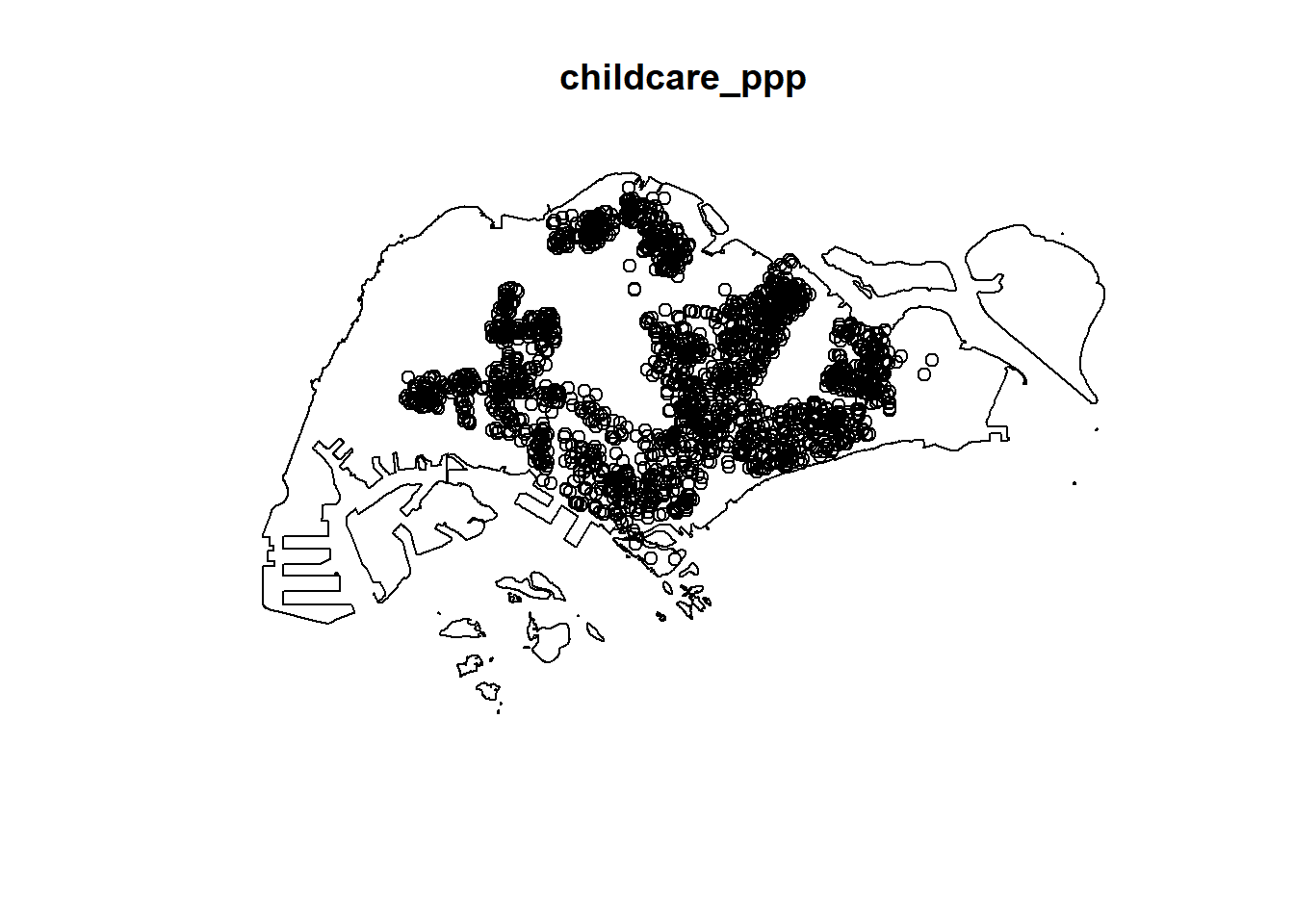

Let’s reveal the properties of the newly created ppp objects using summary().

code chunk

summary(childcare_ppp)

Marked planar point pattern:  1925 points
Average intensity 2.461811e-06 points per square unit

*Pattern contains duplicated points*

Coordinates are given to 11 decimal places

marks are numeric, of type 'double'
Summary:
   Min. 1st Qu.  Median    Mean 3rd Qu.    Max. 
      0       0       0       0       0       0 

Window: polygonal boundary
80 separate polygons (35 holes)
                  vertices         area relative.area
polygon 1            14650  6.97996e+08      8.93e-01
polygon 2 (hole)         3 -2.21090e+00     -2.83e-09
polygon 3              285  1.61128e+06      2.06e-03
polygon 4 (hole)         3 -2.05920e-03     -2.63e-12
polygon 5 (hole)         3 -8.83647e-03     -1.13e-11
polygon 6              668  5.40368e+07      6.91e-02
polygon 7               44  2.26577e+03      2.90e-06
polygon 8               27  1.50315e+04      1.92e-05
polygon 9              711  1.28815e+07      1.65e-02
polygon 10 (hole)       36 -4.01660e+04     -5.14e-05
polygon 11 (hole)      317 -5.11280e+04     -6.54e-05
polygon 12 (hole)        3 -3.41405e-01     -4.37e-10
polygon 13 (hole)        3 -2.89050e-05     -3.70e-14
polygon 14              77  3.29939e+05      4.22e-04
polygon 15              30  2.80002e+04      3.58e-05
polygon 16 (hole)        3 -2.83151e-01     -3.62e-10
polygon 17              71  8.18750e+03      1.05e-05
polygon 18 (hole)        3 -1.68316e-04     -2.15e-13
polygon 19 (hole)       36 -7.79904e+03     -9.97e-06
polygon 20 (hole)        4 -2.05611e-02     -2.63e-11
polygon 21 (hole)        3 -2.18000e-06     -2.79e-15
polygon 22 (hole)        3 -3.65501e-03     -4.67e-12
polygon 23 (hole)        3 -4.95057e-02     -6.33e-11
polygon 24 (hole)        3 -3.99521e-02     -5.11e-11
polygon 25 (hole)        3 -6.62377e-01     -8.47e-10
polygon 26 (hole)        3 -2.09065e-03     -2.67e-12
polygon 27              91  1.49663e+04      1.91e-05
polygon 28 (hole)       26 -1.25665e+03     -1.61e-06
polygon 29 (hole)      349 -1.21433e+03     -1.55e-06
polygon 30 (hole)       20 -4.39069e+00     -5.62e-09
polygon 31 (hole)       48 -1.38338e+02     -1.77e-07
polygon 32 (hole)       28 -1.99862e+01     -2.56e-08
polygon 33              40  1.38607e+04      1.77e-05
polygon 34 (hole)       40 -6.00381e+03     -7.68e-06
polygon 35 (hole)        7 -1.40545e-01     -1.80e-10
polygon 36 (hole)       12 -8.36709e+01     -1.07e-07
polygon 37              45  2.51218e+03      3.21e-06
polygon 38             142  3.22293e+03      4.12e-06
polygon 39             148  3.10395e+03      3.97e-06
polygon 40              75  1.73526e+04      2.22e-05
polygon 41              83  5.28920e+03      6.76e-06
polygon 42             211  4.70521e+05      6.02e-04
polygon 43             106  3.04104e+03      3.89e-06
polygon 44             266  1.50631e+06      1.93e-03
polygon 45              71  5.63061e+03      7.20e-06
polygon 46              10  1.99717e+02      2.55e-07
polygon 47             478  2.06120e+06      2.64e-03
polygon 48             155  2.67502e+05      3.42e-04
polygon 49            1027  1.27782e+06      1.63e-03
polygon 50 (hole)        3 -1.16959e-03     -1.50e-12
polygon 51              65  8.42861e+04      1.08e-04
polygon 52              47  3.82087e+04      4.89e-05
polygon 53               6  4.50259e+02      5.76e-07
polygon 54             132  9.53357e+04      1.22e-04
polygon 55 (hole)        3 -3.23310e-04     -4.13e-13
polygon 56               4  2.69313e+02      3.44e-07
polygon 57 (hole)        3 -1.46474e-03     -1.87e-12
polygon 58            1045  4.44510e+06      5.68e-03
polygon 59              22  6.74651e+03      8.63e-06
polygon 60              64  3.43149e+04      4.39e-05
polygon 61 (hole)        3 -1.98390e-03     -2.54e-12
polygon 62 (hole)        4 -1.13774e-02     -1.46e-11
polygon 63              14  5.86546e+03      7.50e-06
polygon 64              95  5.96187e+04      7.62e-05
polygon 65 (hole)        4 -1.86410e-02     -2.38e-11
polygon 66 (hole)        3 -5.12482e-03     -6.55e-12
polygon 67 (hole)        3 -1.96410e-03     -2.51e-12
polygon 68 (hole)        3 -5.55856e-03     -7.11e-12
polygon 69             234  2.08755e+06      2.67e-03
polygon 70              10  4.90942e+02      6.28e-07
polygon 71             234  4.72886e+05      6.05e-04
polygon 72 (hole)       13 -3.91907e+02     -5.01e-07
polygon 73              15  4.03300e+04      5.16e-05
polygon 74             227  1.10308e+06      1.41e-03
polygon 75              10  6.60195e+03      8.44e-06
polygon 76              19  3.09221e+04      3.95e-05
polygon 77             145  9.61782e+05      1.23e-03
polygon 78              30  4.28933e+03      5.49e-06
polygon 79              37  1.29481e+04      1.66e-05
polygon 80               4  9.47108e+01      1.21e-07
enclosing rectangle: [2667.54, 56396.44] x [15748.72, 50256.33] units
                     (53730 x 34510 units)
Window area = 781945000 square units
Fraction of frame area: 0.422

4 Creating owin object from sf data.frame

We can use as.owin() of spatstat.geom package to create an owin object layer directly from a sf tibble data.frame.

code chunk

sg_owin <- as.owin(sg_sf)
plot(sg_owin)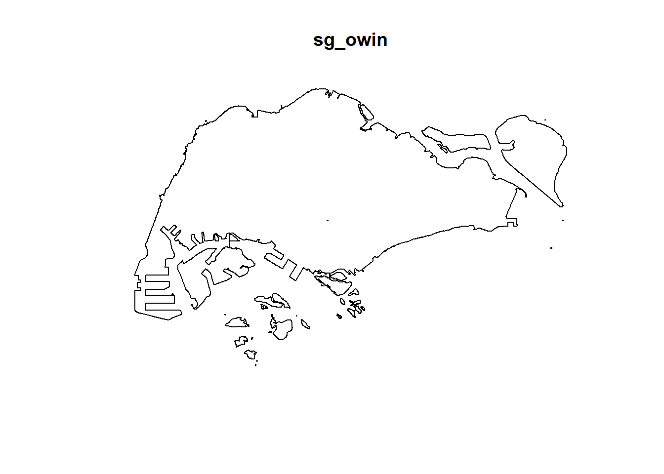

Let’s reveal the properties of the newly created owin objects using summary().

code chunk

summary(sg_owin)

Window: polygonal boundary
80 separate polygons (35 holes)
                  vertices         area relative.area
polygon 1            14650  6.97996e+08      8.93e-01
polygon 2 (hole)         3 -2.21090e+00     -2.83e-09
polygon 3              285  1.61128e+06      2.06e-03
polygon 4 (hole)         3 -2.05920e-03     -2.63e-12
polygon 5 (hole)         3 -8.83647e-03     -1.13e-11
polygon 6              668  5.40368e+07      6.91e-02
polygon 7               44  2.26577e+03      2.90e-06
polygon 8               27  1.50315e+04      1.92e-05
polygon 9              711  1.28815e+07      1.65e-02
polygon 10 (hole)       36 -4.01660e+04     -5.14e-05
polygon 11 (hole)      317 -5.11280e+04     -6.54e-05
polygon 12 (hole)        3 -3.41405e-01     -4.37e-10
polygon 13 (hole)        3 -2.89050e-05     -3.70e-14
polygon 14              77  3.29939e+05      4.22e-04
polygon 15              30  2.80002e+04      3.58e-05
polygon 16 (hole)        3 -2.83151e-01     -3.62e-10
polygon 17              71  8.18750e+03      1.05e-05
polygon 18 (hole)        3 -1.68316e-04     -2.15e-13
polygon 19 (hole)       36 -7.79904e+03     -9.97e-06
polygon 20 (hole)        4 -2.05611e-02     -2.63e-11
polygon 21 (hole)        3 -2.18000e-06     -2.79e-15
polygon 22 (hole)        3 -3.65501e-03     -4.67e-12
polygon 23 (hole)        3 -4.95057e-02     -6.33e-11
polygon 24 (hole)        3 -3.99521e-02     -5.11e-11
polygon 25 (hole)        3 -6.62377e-01     -8.47e-10
polygon 26 (hole)        3 -2.09065e-03     -2.67e-12
polygon 27              91  1.49663e+04      1.91e-05
polygon 28 (hole)       26 -1.25665e+03     -1.61e-06
polygon 29 (hole)      349 -1.21433e+03     -1.55e-06
polygon 30 (hole)       20 -4.39069e+00     -5.62e-09
polygon 31 (hole)       48 -1.38338e+02     -1.77e-07
polygon 32 (hole)       28 -1.99862e+01     -2.56e-08
polygon 33              40  1.38607e+04      1.77e-05
polygon 34 (hole)       40 -6.00381e+03     -7.68e-06
polygon 35 (hole)        7 -1.40545e-01     -1.80e-10
polygon 36 (hole)       12 -8.36709e+01     -1.07e-07
polygon 37              45  2.51218e+03      3.21e-06
polygon 38             142  3.22293e+03      4.12e-06
polygon 39             148  3.10395e+03      3.97e-06
polygon 40              75  1.73526e+04      2.22e-05
polygon 41              83  5.28920e+03      6.76e-06
polygon 42             211  4.70521e+05      6.02e-04
polygon 43             106  3.04104e+03      3.89e-06
polygon 44             266  1.50631e+06      1.93e-03
polygon 45              71  5.63061e+03      7.20e-06
polygon 46              10  1.99717e+02      2.55e-07
polygon 47             478  2.06120e+06      2.64e-03
polygon 48             155  2.67502e+05      3.42e-04
polygon 49            1027  1.27782e+06      1.63e-03
polygon 50 (hole)        3 -1.16959e-03     -1.50e-12
polygon 51              65  8.42861e+04      1.08e-04
polygon 52              47  3.82087e+04      4.89e-05
polygon 53               6  4.50259e+02      5.76e-07
polygon 54             132  9.53357e+04      1.22e-04
polygon 55 (hole)        3 -3.23310e-04     -4.13e-13
polygon 56               4  2.69313e+02      3.44e-07
polygon 57 (hole)        3 -1.46474e-03     -1.87e-12
polygon 58            1045  4.44510e+06      5.68e-03
polygon 59              22  6.74651e+03      8.63e-06
polygon 60              64  3.43149e+04      4.39e-05
polygon 61 (hole)        3 -1.98390e-03     -2.54e-12
polygon 62 (hole)        4 -1.13774e-02     -1.46e-11
polygon 63              14  5.86546e+03      7.50e-06
polygon 64              95  5.96187e+04      7.62e-05
polygon 65 (hole)        4 -1.86410e-02     -2.38e-11
polygon 66 (hole)        3 -5.12482e-03     -6.55e-12
polygon 67 (hole)        3 -1.96410e-03     -2.51e-12
polygon 68 (hole)        3 -5.55856e-03     -7.11e-12
polygon 69             234  2.08755e+06      2.67e-03
polygon 70              10  4.90942e+02      6.28e-07
polygon 71             234  4.72886e+05      6.05e-04
polygon 72 (hole)       13 -3.91907e+02     -5.01e-07
polygon 73              15  4.03300e+04      5.16e-05
polygon 74             227  1.10308e+06      1.41e-03
polygon 75              10  6.60195e+03      8.44e-06
polygon 76              19  3.09221e+04      3.95e-05
polygon 77             145  9.61782e+05      1.23e-03
polygon 78              30  4.28933e+03      5.49e-06
polygon 79              37  1.29481e+04      1.66e-05
polygon 80               4  9.47108e+01      1.21e-07
enclosing rectangle: [2667.54, 56396.44] x [15748.72, 50256.33] units
                     (53730 x 34510 units)
Window area = 781945000 square units
Fraction of frame area: 0.422

5 Combining point events object and owin object

Now we’ll create an ppp object by combining childcare_ppp and sg_owin then plot the output.

code chunk

childcareSG_ppp = childcare_ppp[sg_owin]
plot(childcareSG_ppp)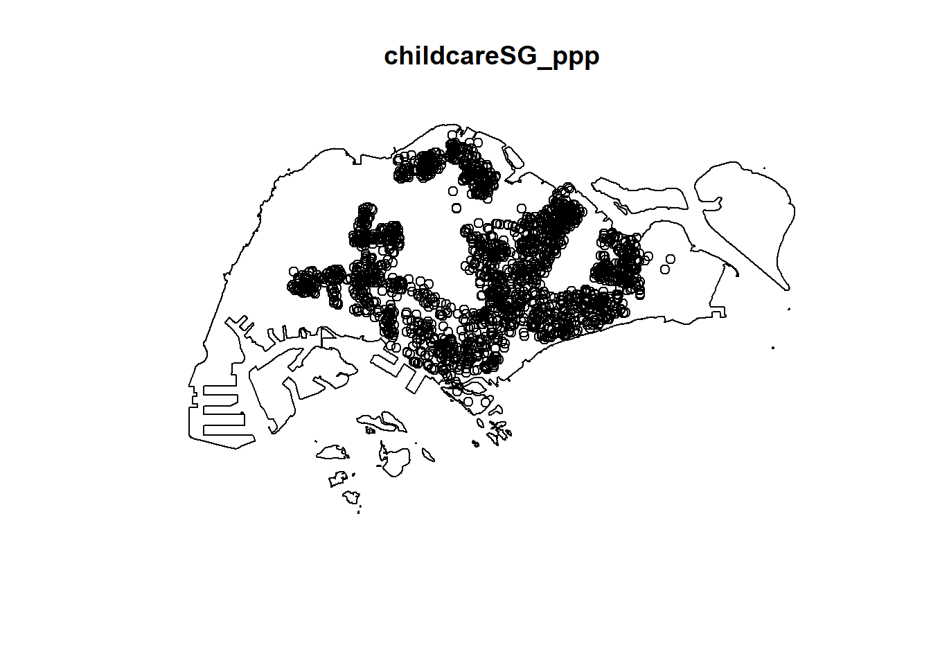

6 Kernel Density Estimation of Spatial Point Event

Before performing Kernel Density Estimation, we need to re-scale the unit of measurement from meter to kilometer.

code chunk

childcareSG_ppp.km <- rescale.ppp(childcareSG_ppp, 
                                  1000, 
                                  "km")

kde_childcareSG_adaptive <- adaptive.density(
  childcareSG_ppp.km, 
  method="kernel")
plot(kde_childcareSG_adaptive)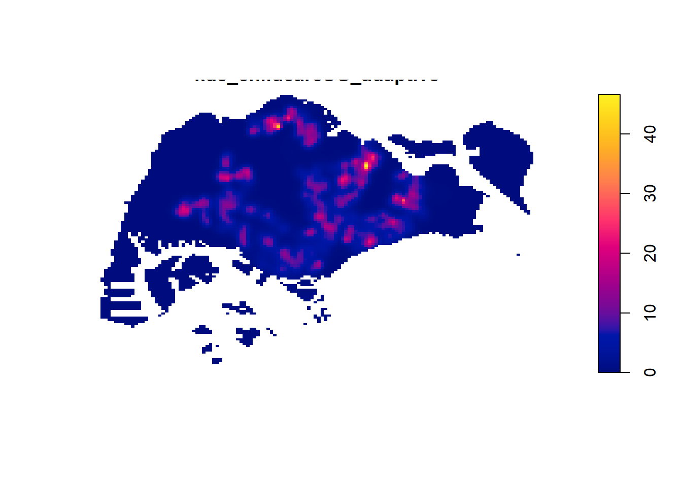

7 Kernel Density Estimation

There are two ways to convert KDE output into grid object

maptools method
spatstat.geom method

code chunk

library(spatstat.geom)
library(raster)
library(sp)

# Set background color
par(bg = '#E4D5C9')

# Convert spatstat image to raster
r <- raster(kde_childcareSG_adaptive)

# Convert raster to SpatialGridDataFrame
gridded_kde_childcareSG_ad <- as(r, "SpatialGridDataFrame")

# Plot using spplot
spplot(gridded_kde_childcareSG_ad)

code chunk

gridded_kde_childcareSG_ad <- as(
  kde_childcareSG_adaptive,
  "SpatialGridDataFrame")
spplot(gridded_kde_childcareSG_ad)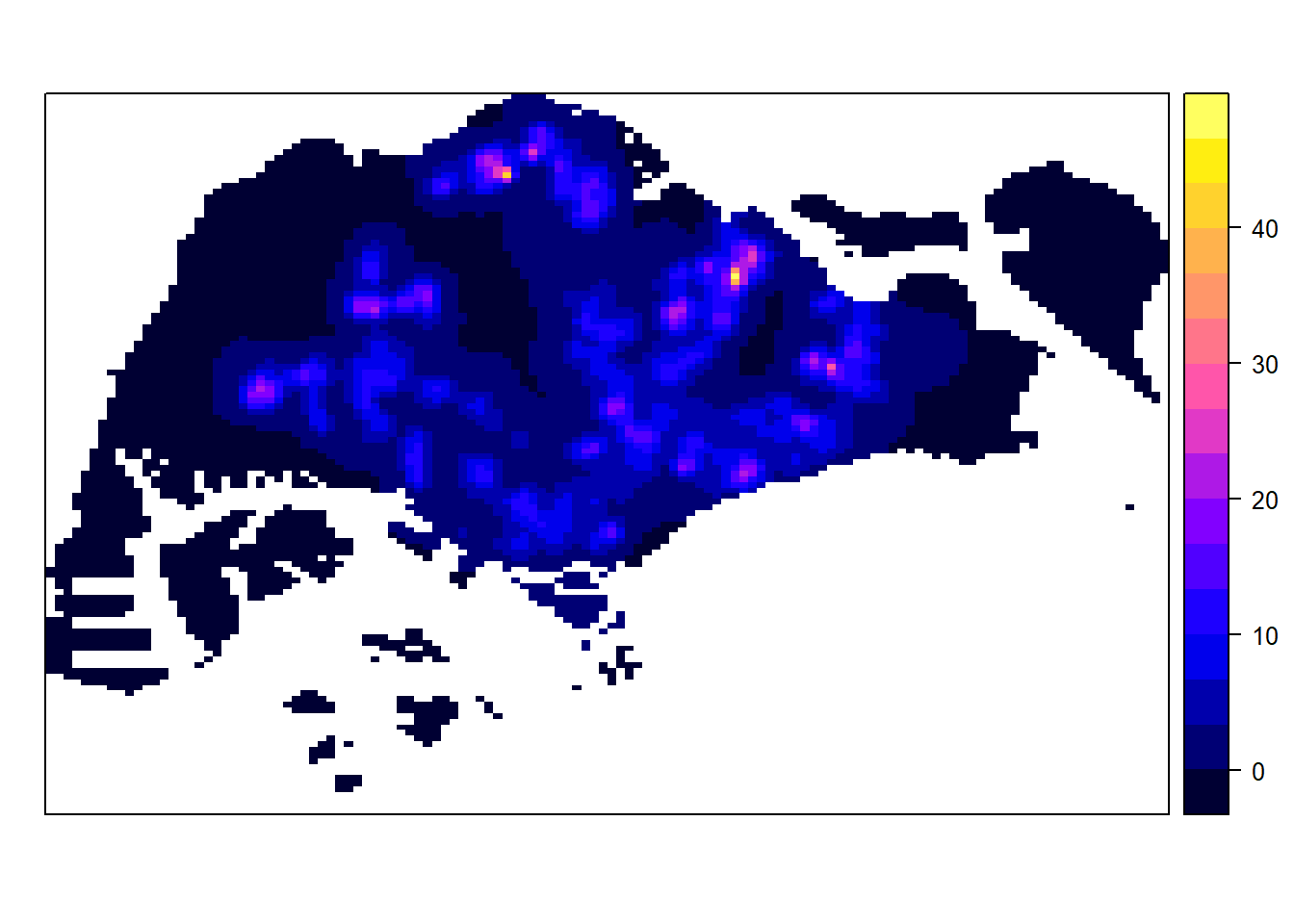

7.1 Visualising KDE using `tmap`

We can plot the output raster by using tmap functions.

code chunk

kde_childcareSG_ad_raster <- raster(gridded_kde_childcareSG_ad)
projection(kde_childcareSG_ad_raster) <- CRS("+init=EPSG:3414")

code chunk

tm_shape(kde_childcareSG_ad_raster) + 
  tm_raster(palette = "viridis") +
  tm_layout(legend.position = c("right", "bottom"), 
            frame = FALSE,
            bg.color = "#E4D5C9")

── tmap v3 code detected ───────────────────────────────────────────────────────

[v3->v4] `tm_tm_raster()`: migrate the argument(s) related to the scale of the
visual variable `col` namely 'palette' (rename to 'values') to col.scale =
tm_scale(<HERE>).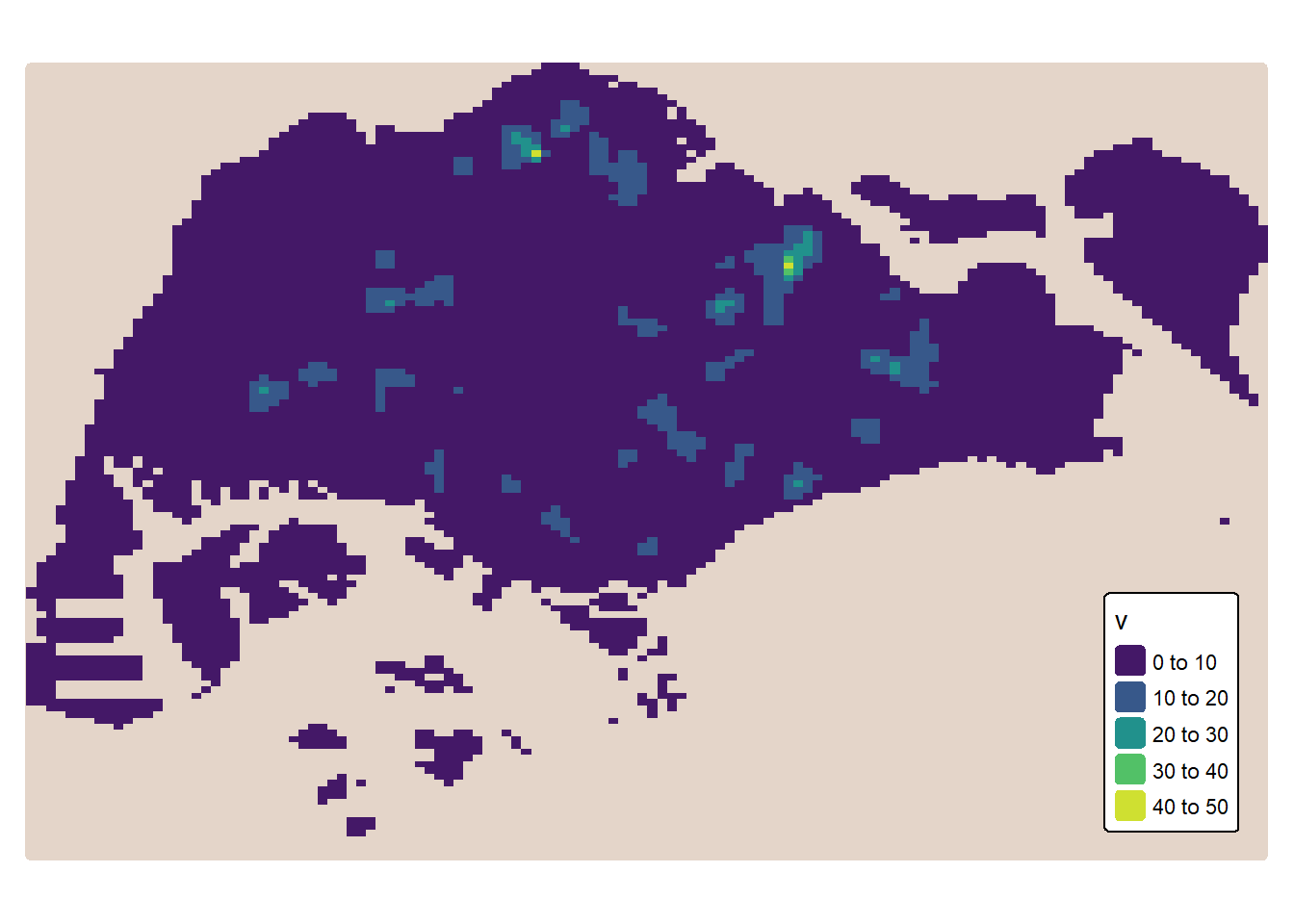

8 Monte Carlo Simulation

In order to ensure reproducibility, it is important to include the code chunk below before using spatstat functions involve Monte Carlo simulation

code chunk

set.seed(2024)

9 Reference

Kam, T. S. In-class Exercise 2: Spatial Point Patterns Analysis: spatstat methods. ISSS626 Geospatial Analytics and Applications.

https://isss626-ay2025-26aug.netlify.app/lesson/lesson02/lesson02-sppa

1 Installing and loading R packages

1.1 Install maptools package

1.2 Install remaining packages

2 The data

2.1 working with st_union()

3 Creating ppp objects from sf data.frame

4 Creating owin object from sf data.frame

5 Combining point events object and owin object

6 Kernel Density Estimation of Spatial Point Event

7 Kernel Density Estimation

7.1 Visualising KDE using tmap

8 Monte Carlo Simulation

9 Reference

2.1 working with `st_union()`

7.1 Visualising KDE using `tmap`